The Thirty-Third AAAI Conference on Artificial Intelligence (AAAI-19)
Compressing Recurrent Neural Networks with Tensor Ring for Action Recognition
Yu Pan,
1Jing Xu,
1Maolin Wang,
1Jinmian Ye,
1Fei Wang,
2Kun Bai,
3Zenglin Xu
1∗ 1University of Electronic Science and Technology of China, Sichuan, ChinaEmails:{ypyupan, xujing.may, morin.w98, jinmian.y, zenglin}@gmail.com 2Weill Cornell Medical College, Cornell University, New York, NY, USA
Email:[email protected]
3Mobile Internet Group, Tencent Inc., Shenzhen, Guangdong, China
Email: [email protected]
Abstract
Recurrent Neural Networks (RNNs) and their variants, such as Long-Short Term Memory (LSTM) networks, and Gated Recurrent Unit (GRU) networks, have achieved promising performance in sequential data modeling. The hidden layers in RNNs can be regarded as the memory units, which are helpful in storing information in sequential contexts. How-ever, when dealing with high dimensional input data, such as video and text, the input-to-hidden linear transformation in RNNs brings high memory usage and huge computational cost. This makes the training of RNNs very difficult. To ad-dress this challenge, we propose a novel compact LSTM model, named as TR-LSTM, by utilizing the low-rank tensor ring decomposition (TRD) to reformulate the input-to-hidden transformation. Compared with other tensor decomposition methods, TR-LSTM is more stable. In addition, TR-LSTM can complete an end-to-end training and also provide a fun-damental building block for RNNs in handling large input data. Experiments on real-world action recognition datasets have demonstrated the promising performance of the pro-posed TR-LSTM compared with the tensor-train LSTM and other state-of-the-art competitors.
Introduction
Recurrent Neural Networks (RNNs) have achieved great success in analyzing sequential data in various applications, such as computer vision (Byeon et al. 2015; Liang et al. 2016; Theis and Bethge 2015), natural language process-ing, etc.. Thanks to the ability in capturing long-range de-pendencies from input sequences (Rumelhart, Hinton, and Williams 1988; Sutskever, Vinyals, and Le 2014). To address the gradient vanishing issue which often leads to the fail-ure of long-term memory in vanilla RNNs, advanced vari-ants such as Gate Recurrent Unit (GRU) and Long-Short Term Memory (LSTM) have been proposed and applied in many learning tasks (Byeon et al. 2015; Liang et al. 2016; Theis and Bethge 2015).
Despite the success, LSTMs and GRUs suffer from the huge number of parameters, which makes the training pro-cess notoriously difficult and easily over-fitting. In particu-lar, in the task of action recognition from videos, a video frame usually forms a high-dimensional input, which makes
Copyright c2019, Association for the Advancement of Artificial Intelligence (www.aaai.org). All rights reserved.
the size of the input-to-hidden matrix extremely large. For example, in the UCF11 (Liu, Luo, and Shah 2009), a video action recognition dataset, an RGB video clip is a frame with a size of160×120×3, and the dimension of the input vec-tor fed to the vanilla RNN can be over 57,000. Assume that the length of hidden layer vector is 256. Then, the input-to-hidden layer matrix has a load of parameters up to 14 mil-lions. Although a pre-processing feature extraction step via deep convolutional neural networks can be utilized to obtain static feature maps as inputs to RNNs (Donahue et al. 2015), the over-parametric problem is still not fully solved.
A promising direction to reduce the parameter size is to explore the low-rank structures in the weight matrices. In-spired from the success of tensor decomposition methods in CNNs (Novikov et al. 2015; Li et al. 2017), various tensor decomposition methods have been explored in RNNs (Yang, Krompass, and Tresp 2017; Ye et al. 2018). In particular, in (Yang, Krompass, and Tresp 2017), the tensor train (TT) de-composition has been applied to RNNs in an end-to-end way to replace the input-to-hidden matrix, and achieved state-of-the-art performance in finding the low-rank structure in RNNs. However, the restricted setting on the ranks and the restrained order of core tensors makes TT-RNN models sen-sitive to parameter selection. In detail, the optimal setting of TT-ranks is that they are small in the border cores and large in middle cores, e.g., like an olive (Zhao et al. 2016).
LSTM with the tensor ring layer, named as TR-LSTM.1 We have conducted empirical evaluations on two real-world action recognition datasets, i.e., UCF11 and HMDB51 (Kuehne et al. 2011). For a fair comparison with standard LSTM and TT-LSTM (Yang, Krompass, and Tresp 2017) and BT-LSTM (Ye et al. 2018), we conduct exper-iments in an end-to-end training. As shown in Figure 7, the proposed TR-LSTM has obtained an accuracy value of 0.869, which outperforms the results of standard LSTM (i.e., 0.681), TT-LSTM (i.e.,0.803), and BT-LSTM (i.e., 0.856). Meanwhile, the compression ratio over the standard LSTM is over 34,000, which is also much higher than the com-pression ratio given by TT-LSTM and BT-LSTM. Moreover, with the output by pre-trained CNN as the input to LSTMs, TR-LSTM has outperformed most previous competitors in-cluding LSTM, TT-LSTM, BT-LSTM, and others recently proposed action recognition methods. Since the TR layer can be used as a building block to other LSTM-based ap-proaches, such as the two-stream LSTM (Gammulle et al. 2017), we believe the proposed TR decomposition can be a promising approach for action recognition, by considering the tricks used in other state-of-the-art methods.
Model
To handle the high dimensional input of RNNs, we intro-duce the tensor ring decomposition to represent the input-to-hidden layer in RNNs in a compact structure. In the follow-ing, we first present preliminaries and background of tensor decomposition, including graphical illustrations of the ten-sor train decomposition and the tenten-sor ring decomposition, followed by our proposed LSTM model, namely, TR-LSTM.
Preliminaries and Background
Notation In this paper, a d-order tensor, e.g., DDD ∈
RL1×L2···×Ld is denoted by a boldface Euler script letter.
With all subscripts fixed, each element of a tensor is ex-pressed as:DDDl1,l2,...ld ∈ R. Given a subset of subscripts,
we can get a sub-tensor. For example, given a subset{L1=
l1, L2=l2}, we can obtain a sub-tensorDDDl1,l2 ∈R
L3···×Ld.
Specifically, we denote a vector by a bold lowercase letter, e.g.,v ∈ RL, and matrices by bold uppercase letters, e.g.,
M ∈ RL1×L2. We regard vectors and matrices as 1-order
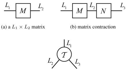
tensors and 2-order tensors, respectively. Figure 1 draws the tensor diagrams presenting the graphical notations and the essential operations.
Tensor Contraction Tensor contraction can be performed between two tensors if some of their dimensions are matched. For example, given two 3-order tensors AAA ∈
RL1×L2×L3 andBBB∈
RJ1×J2×J3, whenL
3 =J1, the con-traction between these two tensors result in a tensor with the size ofL1×L2×J2×J3, where the matching dimension is reduced, as shown in Equation (1):
(AAABBB)l1,l2,j2,j3 =AAAl1,l2BBBj2,j3 = L3
X
p=1 A
AAl1,l2,pBBBp,j2,j3 (1)
1
Note that the tensor ring layer can also be plugged in the vanilla RNN and GRU.
M
L
1L
2(a) aL1×L2matrix
M
L
1N
L
3L
2(b) matrix contraction
L
1L
2L
3(c) aL1×L2×L3tensor
Figure 1: Tensor diagrams. (a) shows the graphical repre-sentation of the matrix M ∈ RL1×L2, where L
1 andL2 denote the matrix size. A matrix is represented by a rect-angular node. (b) demonstrates the contraction between two matrices(tensors), which is represented by an axis connect-ing them together and the contraction between M and N
resulting in a new matrix with shapeRL1×L3. (c) presents
the graphical notation of a tensorTTT ∈RL1×L2×L3.
( )2
. . .
( )d1
( )1
( )dL
d1L
2L
dL
1Rd1
R1
Figure 2: Tensor Train Decomposition: Noted that in tensor train the rankR0andRdare constrained to 1, so the first and
the last core are matrices while the inner cores are 3-order tensors.
Tensor Train Decomposition Through the tensor train decomposition (TTD), a high-order tensor can be decom-posed as the product of a sequence of low-order tensors. For example, ad-order tensorDDD∈RL1×L2···×Ldcan be
decom-posed as follows:
DDDl1,l2,...,ld
T T D
= GGG(1)l
1 GGG
(2)
l2 . . .GGG
(d)
ld
= X
r1,r2,...,rd−1
GGG(1)
r0,l1,r1. . .GGG
(d)
rd−1,ld,rd (2)
where each GGG(k) ∈ RRk−1×Lk×Rk is called a core
tensor. The tensor train rank, shorted as TT-rank, [R0, R1, R2, . . . , Rd], for eachk∈ {0,1, . . . , d},0< rk≤
Rk, corresponds to the complexity of tensor train
decom-position. Generally, in tensor train decomposition, the con-straintR0=Rd= 1should be satisfied and other ranks are
chosen manually. Figure 2 illustrates the form of tensor train decomposition.
. . .
( )d
( )1 ( )2
( )d1
L
2L
dL
1 R1Rd1 R0
L
d1(a) TRD in a ring form
( )2
. . .
( )d 1
r0=2
1
( )
rd=2
d ( )
+
. . .
+
( )2
. . .
( )d 1
rd=R d ( )
r0=R
1
( )
( )2
. . .
( )d1
rd=1d
( )
r0=1 1 ( )
+
L
d1L
2L
dL
1L
d1L
2L
dL
1L
d1L
2L
dL
1}
R
R1
R1
R1
Rd1
Rd1
Rd1
(b) TRD as the sum of TTs (r0=rd)
Figure 3: Two representations of tensor ring decomposition (TRD). In Figure 3(a), TRD is expounded in the traditional way: the core tensors are multiplied one by one, and form a ring structure. In Figure 3(b), TRD is illustrated in an al-ternative way: the summation of a series of tensor trains. By fixing the subscriptr0ofGGG(1) andrdofGGG(d):r0=rd=k,
wherek∈ {1,2, . . . , R}, bothGGG(1)andGGG(d)are divided into
Rmatrices.
the optimized TT cores, but it is still a challenging issue in finding the best alignment(Zhao et al. 2016).
In the tensor ring decomposition(TRD), an important modification is interconnecting the first and the last core ten-sors circularly and constructing a ring-like structure to alle-viate the aforementioned limitations of the tensor train. For-mally, we setR0 =Rd =RandR ≥1, and conduct the
decomposition as:
D
DDl1,l2,...,ld
T RD
= X
r0=rd,r2,...,rd−1
GGG(1)
r0,l1,r1GGG
(2)
r1,l2,r2. . .GGG
(d)
rd−1,ld,rd (3)
For a d-order tensor, by fixing the index k wherek ∈ {1,2, . . . , R}, the first order of the beginning core tensor GGG(1)
r0=k and the last order of the ending core tensorGGG
(d)
rd=k,
can be reduced to matrices. Thus, along each of the R
slices ofGGG(1), we can separate the tensor ring structure as a summation ofRof tensor trains. For example, by fixing
r0=rd=k, the product ofGGG
(1)
k,l1GGG
(2)
l2 . . .GGG
(d)
ld,khas the form
tensor train decomposition. Therefore, the tensor ring model
O 1
. . .
. . . .
I1 I2 In Om O1( )1
( )2
( )n
( )n+1 ( )n+2 ( )n+m
O2
. . .
. . .
input weights output
y x
I
1
Figure 4: TRL: XXX represents the input tensor with shape
RI1×I2×,...,×In after reshaping the input vectorx ∈ RI×1.
By performing the multiplication operation shown in Equa-tion (6) with the weights in TRD form, the output tensor YYYwith shapeRO1×O2×,...,×Omcan be obtained. Then, after
transformingYYYinto vector, we can get the final output vector
y∈RO.
is essentially the linear combination of R different tensor train models. Figure 3 demonstrates the tensor ring structure, and the alternative interpretation as a summation of multiple tensor train structures.
TR-RNN model
The core conception of our model is elaborated in this sec-tion. By transforming the input-to-hidden weight matrices in TR form, and applying them into RNN and its variants, we get our TR-RNN models.
Tensorizingx,y andW Without loss of generality, we tensorize the input vectorx ∈ RI, output vectory ∈ RO,
and weight matrix W ∈ RI×O into tensorsXXX,YYY, andWWW,
shown in Equation (4):
X
XX∈RI1×I2×,...,×In,YYY∈RO1×O2×,...,×Om
WWW∈RI1×I2×,...,×In×O1×O2,...,×Om (4)
where
n
Y
i=1
Ii=I, m
Y
j=1
Oj =O
DecomposingW For an n-order input andm-order out-put, we decompose the weight tensor into the form of TRD with n+m core tensors multiplied one by one, each of which is corresponding to an input dimension or an output dimension, referring to Equation (5). Without loss of gener-ality, the core tensors corresponding to the input dimensions and output dimensions are grouped respectively, as shown in Figure 4.
T RD(WWW)i1,...,in,o1,...,om =
X
r0,...,rn,rn+1,...,rn+m−1
GGG(1)
r0,i1,r1. . .GGG
(n)
rn−1,in,rnGGG
(n+1)
rn,o1,rn+1. . .GGG
(n+m)
The tensor contraction from input to hidden layer in TR form is shown in Equation (6). We multiply the input tensor with input core tensors and output core tensors sequentially. The complexity analysis of forward and backward process is elaborated in the appendix.
YYYo1,o2,...,om =
X
i1,...,in
X X
Xi1,...,inT RD(WWW)i1,...,in,o1,...,om
(6)
Compared with the redundant input-to-hidden weight ma-trix, the compression ratio in TR form is shown in Equa-tion (7).
CT RD =
Qi=n
i=1IiQ j=m j=1 Oj
Pn
i=1Ri−1IiRi+P m
j=1Rn+j−1OjRn+j
(7)
Tensor Ring Layer (TRL) After reshaping the input vec-torxand the weight matrixWinto tensor, and decomposing weight tensor into TR representation, we can get the output tensorYYYby manipulatingWWWandXXX. The final output vec-torycan be obtained by reshaping the output tensorYYYinto vector. Because the weight matrix is factorized with TRD, we denote the whole calculation from the input vectorxto output vectoryas tensor ring layer (TRL):
y=T RL(W,x) (8)
which is illustrated in Figure 4.
TR-RNN By replacing the multiplication between weight matrixWhxand input vectorxwith TRL in vanilla RNN.
We get our TR-RNN model. The hidden state at timetcan be expressed as:
ht=σ(T RL(Whx,xt) +Uhhht−1+b) (9)
whereσ(·)denotes the sigmoid function and the hidden state is denoted byht. The input-to-hidden layer weight matrix
is denoted byWhx, andUhhdenotes the hidden-to-hidden
layer matrix.
TR-LSTM By applying TRL to the standard LSTM, which is the state-of-the-art variant of RNN, we can get the TR-LSTM model as follows.
kt=σ(T RL(Wkx,xt) +Ukhht−1+bk)
ft=σ(T RL(Wf x,xt) +Uf hht−1+bf)
ot=σ(T RL(Wox,xt) +Uohht−1+bo)
gt= tanh(T RL(Wgx,xt) +Ughht−1+bg)
ct=ftct−1+ktgt
ht=ottanh(ct), (10)
where,σ(·)andtanh(·)denote the element-wise product, the sigmoid function and the hyperbolic function, respec-tively. The weight matricesW∗x(where∗can bek, f, o,or
g) denote the mapping from the input to hidden matrix, for the input gatekt, the forget gateft, the output gateot, and
the cell update vectorct, respectively. The weight matrice
U∗hare defined similarly for the hidden stateht−1.
Remark. As shown in Equation (6) and demonstrated in Figure 4, the multiplication between the input tensor
data Xand the input core tensors G(i) (for i = 1, . . . , n) will produce a hidden matrix in the size of R0 ×Rn. It
is important to note that the size of the hidden matrix is much smaller than the original data size. In some sense, the “compressed” hidden matrix can be regarded as the information bottleneck (Tishby, Pereira, and Bialek 2000; Shwartz-Ziv and Tishby 2017), which seeks to achieve the balance between maximally compressing the input informa-tion and preserving the predicinforma-tion informainforma-tion of the out-put. Thus the proposed TR-LSTM has high potentials to re-duce the redundant information in the high-dimensional in-put while achieving good performance compared with the standard LSTM.
Experiments
To evaluate the proposed TR-LSTM model, we first de-sign a synthetic experiment to validate the advantage of tensor ring decomposition over the tensor train decompo-sition. Through two real-world action recognition datasets, i.e., UCF11(YouTube action dataset) (Liu, Luo, and Shah 2009) and HMDB51 (Kuehne et al. 2011), we evaluate our model from two settings: (1) end-to-end training, where video frames are directly fed into the TR-LSTM; and (2) pre-training to obtain features prior to LSTMs, where a pre-trained CNN was used to extract meaningful low-dimensional features and then forwarded these features to the TR-LSTM. For a fair comparison, we first compare our proposed method with the standard LSTM and previous low-rank decomposition methods, and then with the state-of-the-art action recognition methods.
Synthetic Experiment
To verify the effectiveness of tensor decomposition meth-ods in recover the original weights, we design a synthetic dataset. Given a low-rank weight matrix W ∈ R81×81,
which is illustrated in Figure 5(a). We first sample 3200 ex-amples, and each dimension follows a normal distribution, i.e.,x ∼ N(0,0.5I)whereI∈ R81 is the identity matrix.
We then calculateyaccording toy =Wx+for eachx
where∼N(0, σ2I)is a random Gaussian noise andσ2is the variance. Since theyis generated fromx, the recovered weight matrix should be similar to the ground truth. We use the root mean square error (RMSE) to measure the perfor-mance. Should be noted that since the purpose of this exper-iment is to provide a qualitative and intuitive comparison, we do not add any regularization to the models.
noises in Figure 6. It demonstrates that the weight recovered by the tensor ring model has the best tolerance with respect to various injected noises.
(a) Ground truth W
TR2_1=8
(b) Linear Regression
Model:TR, 2=0.05
(c) Tensor Train (d) Tensor Ring
Figure 5: The illustration on the ground truthWand the re-covered weights from different models. The rere-covered RM-SEs of the linear model, tensor train, and tensor ring, are 0.16, 0.18, and 0.09, respectively.
0.02 0.04 0.06 0.08 0.10 0.12 0.14
20.05
0.10
0.15
0.20
0.25
RMSE
TR TT LR
Figure 6: The illustration on how the RMSEs of the linear re-gression(LR), the tensor ring (TR) and the tensor train (TT) change with added noises.
Experiments on the UCF11 Dataset
The UCF11 dataset contains 1600 video clips of a resolution 320×240divided into 11 action categories (e.g., basketball shooting, biking/cycling, diving, etc.). Each category consist of 25 groups of video, within more than 4 clips in one group. It is a challenging dataset due to large variations in camera motion, object appearance and pose, object scale, cluttered background, and so on.
In this part, we conduct two experiments described as “End-to-End Training” and “Pre-train with CNN” on this dataset. In the “End-to-End Training”, we compare the pro-posed TR-LSTM model with other decomposition models
(eg. TT-LSTM (Yang, Krompass, and Tresp 2017) and BT-LSTM (Ye et al. 2018)) to show the superior performance. And in another experiment, we apply decomposition on a more general model, achieving a better performance with less parameters.
BT-LSTM
TT-LSTM
TR-LSTM
0
10000
20000
30000
40000
Compression Ratio
17414 17554
34192
(a) Compression Ratio
0
100 200 300 400 500 600 700 800
Epoch
0
1
2
3
Train Loss
LSTM BT-LSTM TT-LSTM TR-LSTM
(b) Train Loss
0
100 200 300 400 500 600 700 800
Epoch
0.2
0.4
0.6
0.8
Test Accuracy
LSTM: TOP=0.681 BT-LSTM: TOP=0.856 TT-LSTM: TOP=0.803 TR-LSTM: TOP=0.869
(c) Test Accuracy
Figure 7: The results of “End-to-End Training” on UCF11 dataset. (a) shows the different compression ratio based on the vanilla LSTM. (b) and (c) shows the training and testing details.
sam-ple. We set the hidden layer as 256. So there should be a fully-connected layer of4×57600×256 = 58982400 pa-rameters to achieve the mapping for the standard LSTM.
Table 1: Results of “End-to-End Training” on UCF11 re-ported in literature. TT-LSTM was rere-ported in (Yang, Krompass, and Tresp 2017) while the BT-LSTM was re-ported in (Ye et al. 2018).
Method #Params Accuracy
LSTM 59M 0.697
TT-LSTM 3360 0.796 BT-LSTM 3387 0.853 TR-LSTM 1725 0.869
We compare our model with BT-LSTM and TT-LSTM, while using a standard LSTM as a baseline. The hyper-parameters in BT-LSTM and TT-LSTM are set as an-nounced in their papers. Figure 7(c) shows all decompo-sition methods converging faster than the LSTM. The ac-curacy of BT-LSTM is 0.856 which is much higher than TT-LSTM with 0.803 while the LSTM only gain an accu-racy of 0.681. In our TR-LSTM, the shape of input tensor is4×2×5×8×6×5×3×2, the output tensor’s shape is set as4×4×2×4×2and all the TR-ranks are set as 5 exceptR0 =Rd = 10. Results are compared in Table 1.
With 1725 parameters in our model, about half of TT-LSTM and BT-LSTM with parameters 3360 and 3387 respectively. We gain the top accuracy 0.869, showing the outstanding performance of our model in this experiment.
Table 2: The state-of-the-art performance on UCF11.
Method Accuracy
(Hasan and Roy-Chowdhury 2014) 54.5% (Liu, Luo, and Shah 2009) 71.2% (Ikizler-Cinbis and Sclaroff 2010) 75.2% (Liu, Shyu, and Zhao 2013) 76.1% (Sharma, Kiros, and Salakhutdinov 2015) 85.0% (Wang et al. 2011) 84.2% (Sharma, Kiros, and Salakhutdinov 2015) 84.9% (Cho et al. 2014) 88.0% (Gammulle et al. 2017) 94.6%
CNN + LSTM 92.3%
CNN + TR-LSTM 93.8%
Pre-train with CNN Recently, some methods based on RNNs achieved higher accuracy by using the extracted fea-ture as input vectors in computer vision (Donahue et al. 2015). Compared with using frames as input data, extracted features are more compact. But there is still some room for improving the ability of the models. The over-parametric problem is just partial solved. To get better performance, we use extracted features via the CNN model Inception-V3 as input data to LSTM.
We set the size of the hidden layer as32×64 = 2048, which is consistent with the size of the output via Inception-V3. After using the extracted feature as the inputs of LSTM,
the accuracy of the vanilla LSTM attains 0.923. At the same time, the accuracy of our TR-LSTM model whose ranks are set as 40×60×48×48 achieves 93.8. By replacing the standard LSTM with our model, a compression ratio of 25 can be obtained. We compare some state-of-the-art methods in Table 2 on UCF11. The Two Stream LSTM(Gammulle et al. 2017) with highest accuracy has more than 141M pa-rameters. The TR-LSTM can be used to replace the vanilla LSTMs in the Two Stream LSTM model to reduce the pa-rameters.
Experiments on the HMDB51 Dataset
The HMDB51 dataset is a large collection of realistic videos from various sources, such as movies and web videos. The dataset is composed of 6766 video clips from 51 action cat-egories.
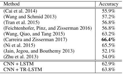
Table 3: Comparison with state-of-the-art results on HMDB51. The best accuracy is 0.664 from the I3D model reported in (Carreira and Zisserman 2017), which bases on 3D ConvNets and is not RNN-based method.
Method Accuracy
(Cai et al. 2014) 55.9% (Wang and Schmid 2013) 57.2% (Tran et al. 2015) 56.8% (Feichtenhofer, Pinz, and Zisserman 2016) 56.8% (Wang, Qiao, and Tang 2015) 63.2% (Carreira and Zisserman 2017) 66.4% (Ni et al. 2015) 65.5% (Jain, Jegou, and Bouthemy 2013) 52.1% (Zhu et al. 2013) 54.0%
CNN + LSTM 62.9%
CNN + TR-LSTM 63.8%
In this experiment, we still use extracted features as the input vector via Inception-V3 and reshape it into64×32. We sample 12 frames from each video clip randomly and be processed through the CNN as the input data. The shape of hidden layer tensor is set as32×64 = 2048. The ranks of our TR-LSTM are40×60×48×48. Some of the state-of-the-art models like I3D (Carreira and Zisserman 2017) are presented in Table 3. The I3D model with highest accuracy based on 3D ConvNets, which is not RNN-based method, has 25M parameters, while the TR-LSTM model only has 0.7M parameters. The TR-LSTM gains a higher accuracy of 63.8% than the standard LSTM with a compressing ratio of 25.
Related Work
methods have improved the classification accuracy, but the over-parametric problem is just still partially solved. In this work, we focus on designing low-rank structure to replace the redundant input-to-hidden weight matrix in RNNs, while compressing the whole model and maintaining the model performance.
The most straight-forward way to apply low-rank con-straint is implementing matrix decomposition on weight ma-trices. Singular Value Decomposition (SVD) has been ap-plied in convolutional neural networks to reduce parame-ters (Denton et al. 2014) but incurred a loss in model per-formance. Besides, the compression ratio is limited because of the rank in matrix decomposition still relatively large.
Compared with matrix decomposition, tensor decomposi-tion (Xu, Yan, and Qi 2015; Zhe et al. 2016; Hao et al. 2018; He et al. 2018; Liu et al. 2018a) conducts data decompo-sition in a higher dimension, capturing higher-order corre-lations while maintaining several orders of fewer parame-ters (Kim et al. 2015; Novikov et al. 2015). Among these methods, (Lebedev et al. 2014) utilized CP decomposition to speed up convolution computation, which has the similar de-sign philosophy with the widely-used depth-wise separable convolutions (Howard et al. 2017). However, the instability issue (de Silva and Lim 2008) hinders the low-rank CP de-composition from solving many important computer vision tasks. (Kim et al. 2015) used Tucker decomposition to de-compose both the convolution layer and the fully connected layer, reducing run-time and energy significantly in mobile applications with minor accuracy drop. Block-Term tensor decomposition combines the CP and Tucker by summing up multiple Tucker models to overcome their drawbacks and has obtained a better performance in RNNs (Ye et al. 2018). However, the computation of the core tensor in the Tucker model is highly inefficient due to the complex tensor flatten and permutation operations. Recent years, the tensor train decomposition also used to substitute the redundant fully connected layer in both CNNs and RNNs (Novikov et al. 2015; Yang, Krompass, and Tresp 2017), preserving the per-formance while reducing the number of parameters signifi-cantly up to 40 times.
But tensor train decomposition has some limitations: 1) certain constraints for TT-rank, i.e., the ranks of the first and last factors are restricted to be 1, limiting its represen-tation power and flexibility. 2) A strict order must be fol-lowed when multiplying TT cores, so that the alignment of the tensor dimensions is extremely important in obtaining the optimized TT cores, but it is still a challenging issue in finding the best alignment. In this paper, we use the Tensor Ring(TR) decomposition (Zhao et al. 2016) to overcome the drawbacks in TTD, while achieving more computation effi-ciency than BT decomposition.
Conclusion
In this paper, we applied TRD to plain RNNs to replace the over-parametric input-to-hidden weight matrix when deal-ing with high-dimensional input data. The low-rank struc-ture of TRD can capstruc-ture the correlation between feastruc-ture di-mensions with fewer orders of magnitude parameters. Our TR-LSTM model achieved best compression ratio with the
highest classification accuracy on UCF11 dataset among other end-to-end training RNNs based on low-rank meth-ods. At the same time, when processing the extracted fea-ture through InceptionV3 as the input vector, our TR-LSTM model can still compress the LSTM while improving the accuracy. We believe that our models provide fundamental modules for RNNs, and can be widely used to handle large input data. In future work, since our models are easy to be extended, we want to apply our models to more advanced RNN structures (Gammulle et al. 2017) to get better perfor-mance.
Acknowledgments
We thank the anonymous reviewers for valuable comments to improve the quality of our paper. This work was par-tially supported by National Natural Science Foundation of China (Nos.61572111 and 61876034), and a Fundamen-tal Research Fund for the Central Universities of China (No.ZYGX2016Z003).
References
Byeon, W.; Breuel, T. M.; Raue, F.; and Liwicki, M. 2015. Scene labeling with lstm recurrent neural networks. In
CVPR, 3547–3555.
Cai, Z.; Wang, L.; Peng, X.; and Qiao, Y. 2014. Multi-view super vector for action recognition. InCVPR, 596–603. IEEE Computer Society.
Carreira, J., and Zisserman, A. 2017. Quo vadis, action recognition? A new model and the kinetics dataset. In
CVPR, 4724–4733. IEEE Computer Society.
Cho, J.; Lee, M.; Chang, H. J.; and Oh, S. 2014. Robust ac-tion recogniac-tion using local moac-tion and group sparsity. Pat-tern Recognition 201447(5):1813–1825.
de Silva, V., and Lim, L. 2008. Tensor rank and the ill-posedness of the best low-rank approximation problem.
SIAM J. Matrix Analysis Applications30(3):1084–1127. Denton, E. L.; Zaremba, W.; Bruna, J.; LeCun, Y.; and Fer-gus, R. 2014. Exploiting linear structure within convo-lutional networks for efficient evaluation. InNIPS, 1269– 1277.
Donahue, J.; Hendricks, L. A.; Guadarrama, S.; Rohrbach, M.; Venugopalan, S.; Darrell, T.; and Saenko, K. 2015. Long-term recurrent convolutional networks for visual recognition and description. InCVPR, 2625–2634. IEEE Computer Society.
Feichtenhofer, C.; Pinz, A.; and Zisserman, A. 2016. Convo-lutional two-stream network fusion for video action recog-nition. InCVPR, 1933–1941. IEEE Computer Society. Gammulle, H.; Denman, S.; Sridharan, S.; and Fookes, C. 2017. Two stream LSTM: A deep fusion framework for hu-man action recognition. InWACV, 177–186. IEEE. Hao, L.; Liang, S.; Ye, J.; and Xu, Z. 2018. Tensord: A tensor decomposition library in tensorflow.Neurocomputing
Hasan, M., and Roy-Chowdhury, A. K. 2014. Incremental activity modeling and recognition in streaming videos. In
CVPR, 796–803. IEEE.
He, L.; Liu, B.; Li, G.; Sheng, Y.; Wang, Y.; and Xu, Z. 2018. Knowledge base completion by variational bayesian neural tensor decomposition.Cognitive Computation.
Howard, A. G.; Zhu, M.; Chen, B.; Kalenichenko, D.; Wang, W.; Weyand, T.; Andreetto, M.; and Adam, H. 2017. Mo-bilenets: Efficient convolutional neural networks for mobile vision applications. CoRRabs/1704.04861.
Ikizler-Cinbis, N., and Sclaroff, S. 2010. Object, scene and actions: Combining multiple features for human action recognition. InECCV, 494–507. Springer.
Jain, M.; Jegou, H.; and Bouthemy, P. 2013. Better exploit-ing motion for better action recognition. In CVPR 2013, 2555–2562. IEEE Computer Society.
Kim, Y.; Park, E.; Yoo, S.; Choi, T.; Yang, L.; and Shin, D. 2015. Compression of deep convolutional neural net-works for fast and low power mobile applications. CoRR
abs/1511.06530.
Kuehne, H.; Jhuang, H.; Garrote, E.; Poggio, T. A.; and Serre, T. 2011. HMDB: A large video database for human motion recognition. InICCV, 2556–2563. IEEE Computer Society.
Lebedev, V.; Ganin, Y.; Rakhuba, M.; Oseledets, I. V.; and Lempitsky, V. S. 2014. Speeding-up convolutional neu-ral networks using fine-tuned cp-decomposition. CoRR
abs/1412.6553.
Li, G.; Ye, J.; Yang, H.; Chen, D.; Yan, S.; and Xu, Z. 2017. Bt-nets: Simplifying deep neural networks via block term decomposition.CoRRabs/1712.05689.
Liang, X.; Shen, X.; Xiang, D.; Feng, J.; Lin, L.; and Yan, S. 2016. Semantic object parsing with local-global long short-term memory. InCVPR, 3185–3193.
Liu, B.; He, L.; Li, Y.; Zhe, S.; and Xu, Z. 2018a. Neuralcp: Bayesian multiway data analysis with neural tensor decom-position.Cognitive Computation.
Liu, H.; He, L.; Bai, H.; Dai, B.; Bai, K.; and Xu, Z. 2018b. Structured inference for recurrent hidden semi-markov model. InIJCAI, 2447–2453.
Liu, J.; Luo, J.; and Shah, M. 2009. Recognizing realistic actions from videos “in the wild”. InCVPR, 1996–2003. IEEE.
Liu, D.; Shyu, M.-L.; and Zhao, G. 2013. Spatial-temporal motion information integration for action detection and recognition in non-static background. InIRI, 626–633. IEEE.
Ni, B.; Moulin, P.; Yang, X.; and Yan, S. 2015. Motion part regularization: Improving action recognition via trajec-tory group selection. InCVPR, 3698–3706. IEEE Computer Society.
Novikov, A.; Podoprikhin, D.; Osokin, A.; and Vetrov, D. P. 2015. Tensorizing neural networks. InNIPS, 442–450. Rumelhart, D. E.; Hinton, G. E.; and Williams, R. J. 1988.
Learning representations by back-propagating errors. Cog-nitive modeling5(3):1.
Sharma, S.; Kiros, R.; and Salakhutdinov, R. 2015. Action recognition using visual attention. CoRRabs/1511.04119. Shwartz-Ziv, R., and Tishby, N. 2017. Opening the black box of deep neural networks via information. CoRR
abs/1703.00810.
Sutskever, I.; Vinyals, O.; and Le, Q. V. 2014. Sequence to sequence learning with neural networks. InNIPS, 3104– 3112.
Theis, L., and Bethge, M. 2015. Generative image modeling using spatial lstms. InNIPS, 1927–1935.
Tishby, N.; Pereira, F. C. N.; and Bialek, W. 2000. The information bottleneck method.CoRRphysics/0004057. Tran, D.; Bourdev, L. D.; Fergus, R.; Torresani, L.; and Paluri, M. 2015. Learning spatiotemporal features with 3d convolutional networks. InICCV, 4489–4497. IEEE Com-puter Society.
Wang, H., and Schmid, C. 2013. Action recognition with improved trajectories. InICCV, 3551–3558. IEEE Com-puter Society.
Wang, H.; Kl¨aser, A.; Schmid, C.; and Liu, C. 2011. Ac-tion recogniAc-tion by dense trajectories. InCVPR, 3169–3176. IEEE.
Wang, L.; Qiao, Y.; and Tang, X. 2015. Action recogni-tion with trajectory-pooled deep-convolurecogni-tional descriptors. InCVPR, 4305–4314. IEEE Computer Society.
Xu, Z.; Yan, F.; and Qi, Y. A. 2015. Bayesian nonparamet-ric models for multiway data analysis. IEEE Trans. Pattern Anal. Mach. Intell.37(2):475–487.
Yang, Y.; Krompass, D.; and Tresp, V. 2017. Tensor-train recurrent neural networks for video classification. InICML, 3891–3900.
Ye, J.; Wang, L.; Li, G.; Chen, D.; Zhe, S.; Chu, X.; and Xu, Z. 2018. Learning compact recurrent neural networks with block-term tensor decomposition. InCVPR.
Zhao, Q.; Zhou, G.; Xie, S.; Zhang, L.; and Cichocki, A. 2016. Tensor ring decomposition.CoRRabs/1606.05535. Zhe, S.; Zhang, K.; Wang, P.; Lee, K.; Xu, Z.; Qi, Y.; and Ghahramani, Z. 2016. Distributed flexible nonlinear tensor factorization. InNIPS, 920–928.