A New Criterion for Lag-Length Selection in Unit Root Tests

(1)

Published online January 30, 2014 (http://www.sciencepublishinggroup.com/j/ajtas) doi: 10.11648/j.ajtas.20130206.28

A new criterion for lag-length selection in unit root tests

Agunloye, Oluokun Kasali

*

; Arnab, Raghunath; Shangodoyin, Dahud Kehinde

Department of Statistics, University of Botswana, Gaborone, Botswana

Email address:

[email protected] (Agunloye O. K.)

To cite this article:

Agunloye, Oluokun Kasali; Arnab, Raghunath; Shangodoyin, Dahud Kehinde. A New Criterion for Lag-Length Selection in Unit Root Tests. American Journal of Theoretical and Applied Statistics. Vol. 2, No. 6, 2013, pp. 293-298. doi: 10.11648/j.ajtas.20130206.28

Abstract:

This paper examines lag selection problem in unit root tests which has become a major specification problem in empirical analysis of non-stationary time series data. It is known that the implementation of unit root tests requires the choice of optimal truncation lag for good power proper ties and it is equally unrealistic to assume that the true optimal truncation lag is known a prior to the practitioners and other applied researchers. Consequently, these users rely largely on the use of standard information criteria for selection of truncation lag in unit root tests. A number of previous studies have shown that these criteria have problem of over-specification of truncation lag-length leading to the well-known low power problem that is commonly associated with most unit root tests in the literature. This paper focuses on the problem of over-specification of truncation lag-length within the context of augmented Dickey-Fuller (ADF) and generalized least squares Dickey-Fuller (DF-GLS)unit root tests. In an attempt to address this lag selection problem, we propose a new criterion for the selection of truncation lag in unit root tests based on Koyck distributed lag model and we show that this new criterion avoids the problem of over-specification of truncationlag-length that is commonly associated with standard information criteria.

Keywords:

Truncation Lag, Information Criteria, Koyck Distributed Lag Model, Unit Root Test, Low Power, Partial Correlation Coefficient

1. Introduction

Testing for the presence of unit root in time series data is a major precondition in any cointegration analysis and other empirical research using time series data. Determination of appropriate truncation lag is quite a challenging aspect of unit root testing. A number of previous studies such as [1], [2], [3],[4],[5] and [6] have shown that there is a strong connection between truncation lag and the empirical power of unit root tests. Among numerous unit root tests proposed in the literature, the augmented Dickey–Fuller (ADF) test introduced by [7] and the generalized least squares Dickey-Fuller (DF-GLS) test introduced by [8] appears to be the most popular unit root tests among applied researchers. Both ADF and DF-GLS unit root tests are well-formulated to handle any possible serial correlations in the error terms of the Dickey–Fuller regressions by augmenting the regressions with lagged differences of the original series. However, the empirical implementation of the ADF and DF-GLS unit root tests requires the inclusion of appropriate number of lagged differences in the Dickey–Fuller regression, which is commonly referred to as lag selection problem in the literature. In practice, lag-lengths are commonly selected by two different lag selection techniques such as

(2)

standard information criteria is the fact that different lag selection criteria choose different optimal truncation lag-lengths for the same dataset. This multiple suggestions of possible truncation lags by different information criteria raises a fundamental question as to on which particular information criterion could we rely upon for the choice of optimal truncation lag-length. To date, there exists no operational procedure for selecting optimal truncation lag-length for unit root tests that gives the best results. Hence, this paper focuses on the choice of optimal truncation lag-length for the ADF family of unit root tests and DF-GLS test since these are the most widely used unit root tests in empirical analysis.

2. Standard Information Criteria

In this study, we considered four standard information criteria for lag selection in unit root testing. The procedure

is to fit autoregressive model on

y

_t

( )

i

,

i

=

1,....,4

for order ranging from 1 to 9 and subsequently obtaining the quantities to compute the values of the criteria. The following lag selection methods are considered:

i.[12]: Final Prediction Error (FPE)

( )

_ˆ2 2 1

(

)

ln _k k

FPE k

N k

σ

+

= +

−

ii.[13]: Akaike Information Criterion(AIC)

( )

_ln _ˆ2 2 1

(

)

k

k AIC k

N

σ +

= +

iii.[14]:Bayesian Information Criterion (BIC)

( )

_ˆ

2

(

1 )

ln

_k

k

N

BIC k

N

σ

+

=

+

iv.[15]: Hannan-Quinn Information Criteria (HQIC)

( )

2 2 1

(

)

ln ln

(

( )

)

ˆ

ln _k k N

HQIC k

N

σ

+

= +

Where

k

is the lag-length selected, N is the sample size and

σ

ˆ

_k2 is the MLE of the model residual. Our objective is to ascertain if these conventional lag selection criteria either over-fit or under-fit the truncation lags by comparing the lag-length suggested by these information criteria with lag-length suggested by the new lag selection criterion.

3. A New Approach to Selection of

Truncation Lag in Unit Root Tests

We consider a distributed lag representation of ADF and DF-GLS regression models in the form:

( )

1

1 1

0

2

1 2

0

3

1 3

0

4

1 4

0

k

t t t j t j t

j

k

t t t j t j t

j

k

t t t j t j t

j

k

d d d

t t t j t j t

j

y

t

y

t

y

ρ

γ

ε

α ρ

γ

ε

α β ρ

γ

ε

α γ

ρ

δ

ε

− −

=

− −

=

− −

=

− −

=



= ∆ −

=

∆

+



= ∆ − −

=

∆

+

_







= ∆ − −

−

=

∆

+



= ∆ − − −

=

∆

+





∑

(1)

Where

y

_t( )1 is ADF Model I with no constant and no trend

( )2

t

y

is ADF Model IIwith constant but no trend

( )3

t

y

is ADF Model III with both constant and trend

( )4

t

y

is DF-GLS with both constant and trend

,

1,..., 4

ti

i

ε =

are white noise error terms,

k

is the truncation lag-length to be determined empirically,

γ

_j and

j

δ

are coefficients of differenced lagged values. The R.H.S of equation (1) is similar to typical distributed lag models used in econometric modeling. [16] has proposed an ingenious method of specifying the lag in distributed lag model by assuming that the coefficients of

i

γ

’s and

δ

_i’s on the R.H.S of equation (1) are all of the same sign and declines geometrically, then without loss of generality we can assume Koyck postulations as follows:

Let

or

k

λ

_

δ

γ

_

 

=

(2)

then we have

( )

0 ki

0,1,

1,....,4

k

λ

R

k

i

λ

=

(3)

Where R is the partial correlation coefficient between

( )

i

_/

_{1,..., 4} t

y

i

= and t j

y

₋

∆

or d

t j y₋

∆ and measures the rate at which ( )i

t

y

depends on either t j y₋

∆ or d t j

y

₋

∆

and for the rate of decline of

k

λ

’s we take _{( )}

i

R such that 0<R_{( )}_i <1

is the indicator of decay of the distributed lag and 1−R_{( )}_i is the speed of adjustment[17].

Equation(2) fundamentally postulates that each

λ

coefficient is a measure of dependence of ( )i

t

(3)

t j

y

₋

∆

or d t j y₋

∆ and each successive

λ

coefficient is

numerically less than each preceding

λ

,this implies that as one goes back into the distant past the effect of that lag on

( )

i

t

y

becomes progressively smaller.

To obtain the mean lag, we ensure that the long-run multiplier is finite

That is the sum of

k

λ is defined as

( ) 0 0 i k k k R

λ

∞ = =

∑

(4)

but

( )i 1 1 _{( )}

i

k

R

=

−

∑

(5)

is the inverse of speed of adjustment. Therefore, the Mean lag is 1 0 0 1 0 1 1 1 i k k L k i k i k i i i k k R k R R kR R λ λ λ λ λ λ                                                                                   = ₋ − = − = = − −

∑

(6)

Applying arithmetic-geometric progression rule to (6) we obtain the sum to infinity for the term

( )i

k

kR

to be

( ) ( ) ( ) 2 0

₁

i i i k k

R

kR

R

        ∞ =

=

₋

∑

₍₇₎

So using (7) in (6) gives

( ) ( ) ( )

,

1,...,5

1

i i i

R

L

i

R

=

₋

=

(8)

The notation ( )i

R

indicates that we generate different R’s for each of the models described in equation (1) and we shall demonstrate the power of test for

( )i

R

for different values of ρ=0.001, 0.5,and 0.999.

The following are the immediate consequences of equation (8) :

(i).The closer R is to +1 ,the slower the rate of decline in

k

λ

,whereas the closer it is to zero, the more rapid the decline in

k

λ

.This ensures that, to have reasonable mean lag

L

_{( )}_i we expect the absolute value of R to be in the

interval

[

0.5, 0.999

)

(ii)The simple linear regression model will be fitted to the L.H.S of equation (1) to generate the parameters needed

and to compute

_y

_t( )i

_,

∀ =

_i

_{1,..., 4}

(iii)If _{( )} 0.3

i

R < _{, then the mean lag will be assumed to be}

zero since ( ) ( ) 1 i i R R        − 

for

R

_{( )}

_i <0.3 is a fraction not up to 0.5.

(iv)The partial correlation coefficient

( )

i

R

should be

computed such that we include all variables and adjusted for maximum lag until it gives a value less than 0.3

4. Power of Test for R

We define power of test for ( )i

R

as follows:

( )

0

:

i

1 H R

=

_against

H R

₁

:

_{( )}_i

<

1

Assuming that

( )

i

R

is normally distributed, then we

define the test statistic as

( )

ˆ

₁

ˆ

i i

R

Z

V R

 

 

−

=

₍₉₎

We reject the null hypothesis of

( ) 1

i

R = and hence leads to

undefined mean lag Lat a specified level of significance

α

if

_Z

< −

_Z

_α.The Power of possible mean lag is the probability of rejecting

0

H

when

H

₁ is true i.e when

( )i 1

R < =R∗

Thus we have

( )

/

_i

P R

 

P Z



Z

_α

R



   

∗

₌

_{< −}

₌

∗ ₍₁₀₎

This reduces to

( )

( ) ( ) ( )

ˆ

₁

/

ˆ

i i i

R

P R

P

Z

R

V R

α ∗ ∗                        

−

=

< −

=

(11)

( )

ˆ

1 _/

ˆ

i i i i

R

P

Z

R

V R

α ∗                      _ _ _ _         

(4)

( )

( ) ( ) ( )

( )

ˆ

1 _/

ˆ

i

i i i

R

_R

P

Z

R

V R

α ∗ ∗ ∗                                

−

=

< − +

−

=

(

)

( )

(

)

( )

1

1 ˆ

ˆ

i i

R

P Z

Z

P Z

Z

V R

α α ∗ ∗                                        

−

=

< − +

=

< − −

(

)

( )

1 ˆ

i

R

P Z

Z

V R

α ∗                    

−

=

>

+

(12)

After some algebraic manipulation of Equation (11) we have Equation (12) which defines the power of test for

( )

i

R

5. Empirical Illustration

For empirical illustration, we fit simulated data to the distributed lag specifications of Dickey-Fuller regression models of ADF and DF-GLS unit root tests as follows:

For ADF MODEL I , ( )1

1 1

0

k

t t t j t j t

j

y y

ρ

y₋

γ

y₋

ε

=

= ∆ − =

∑

∆ +

We set

ρ

=0.001,0.5 and 0.999 in

y

_t( )1 to have the following representations: ( ) 1 1 1 1 2 1 3

0.001* , 0.001

0.5* , 0.5

0.999* , 0.999

t t

t t t

t t

y y a

y y y a

y y a

ρ ρ ρ − − − ∆ − = =    = ∆ − = =   ∆ − = = 

We generate series

a

₁ ,

a

₂ and

a

₃ for different values of

ρ

=

0.001, 0.5 and 0.999

.We compute partial correlation coefficients between :

a

₁ and different choices of variables from the set of independent variables

1 2 12

,

,...,

t t t t

y

₋

y

₋

y

₋

∆ ∆

∆

while controlling for the effects of other remaining independent variables. We also repeat the same procedure for

a

₂ and

a

₃

For ADF MODEL II , ( )2

1 2

0

k

t t t j t j t

j

y y α ρy₋ γ y₋ ε

=

= ∆ − − =

∑

∆ + ,

we set ρ=0.001,0.5 and 0.999 in

y

_t( )2 to have the following representations:

( )

1 1 1

2

2 1 2

3 1 3

0.001* , 0.001

0.5* , 0.5

0.999 * , 0.999

t t

t t t

t t

y y b

y y y b

y y b

α ρ α ρ α ρ − − − ∆ − − = =    = ∆ − − = =   ∆ − − = = 

where

α

₁ ,

α

₂ and

α

₃ are obtained by fitting of a regression model

y

_t( )2 equals to a constant for different values of

ρ

.With values of

α

₁,

α

₂ and

α

₃ known ,we therefore proceed to generate the series for

b

₁ ,

b

₂ and

3

b

.Thereafter, we compute partial correlation coefficient

between :

b

∆ ∆

y

_t

,

y

_t₋₁

,

∆

y

_t₋₂

,...,

∆

y

_t₋₁₂ while controlling for the effects of other remaining independent variables. We also repeat the same procedure for

b

₂ and

b

₃

For ADF MODEL III,

( )3

1 3

0

k

t t t j t j t

j

y y α β ρt y₋ γ y₋ ε

=

= ∆ − − − =

∑

∆ + ,

we set

ρ

=

0.001, 0.5 and 0.999

in

y

_t( )3 to have the following representations:

( )

1 1 1 1

3

2 2 1 2

3 3 1 3

0.001* , 0.001

0.5* , 0.5

0.999* , 0.999

t t

t t t

t t

y t y d

y y t y d

y t y d

α β ρ

− − − ∆ − − − = =    = ∆ − − − = =   ∆ − − − = = 

We estimate the regression equation

( )3

1

*

t t t

y

= +

α β

t

+ ∆ +

y

ρ

y

₋ , for values of

0.001, 0.5 and 0.999

ρ

= .Thereafter, we proceed to generate series for d₁ , d2 and d3 .We compute partial

correlation coefficients between:

d

1 2 12

,

,...,

t t t t

y

₋

y

₋

y

₋

∆ ∆

∆

d

₂ and

d

₃

For DF-GLS unit root test,

( )4

1 4

0

k

d d d

t t t j t j t

j

y y α γ ρt y₋ δ y₋ ε

=

= ∆ − − − =

∑

∆ + ,

we set ρ=0.001,0.5 and 0.999 in

y

t( )4 to have the following representations:

( )

1 1 1 1

4

2 2 1 2

3 3 1 3

0.001* , 0.001

0.5* , 0.5

0.999 * , 0.999

d d

t t

d d

t t t

d d

t t

y t y e

y y t y e

y t y e

α γ ρ

(5)

We estimate the regression equation

( )4

1

* d * d

t t t

y = +

α γ

t+ ∆ +y

ρ

y₋ , for values of

0.001, 0.5 and 0.999

ρ

= .Thereafter, we proceed to generate series for

e

₁ ,

e

₂ and

e

₃ .We compute partial correlation coefficients between:

e

1 2 12

,

,...,

t t t t

y

₋

y

₋

y

₋

∆ ∆

∆

e

₂ and

e

₃

6. Power of Test for ADF and DF-GLS

Unit Root Tests under the New Lag

Selection Criterion

In this section, we discuss the power of test for R for the ADF and DF-GLS unit root tests based on the optimal truncation lag selected by the new criterion.

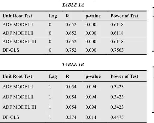
Table 1.Power of Test for R Whenρ=0.001

TABLE 1A

Unit Root Test Lag R p-value Power of Test

ADF MODEL I 0 0.652 0.000 0.6118 ADF MODELII 0 0.652 0.000 0.6118 ADF MODEL III 0 0.652 0.000 0.6118 DF-GLS 0 0.752 0.000 0.7563

TABLE 1B

ADF MODEL I 1 0.054 0.094 0.3423 ADF MODELII 1 0.054 0.094 0.3423 ADF MODEL III 1 0.054 0.094 0.3423 DF-GLS 1 0.374 0.014 0.4475

From Tables 1A and 1B above, it is obvious that the partial correlation coefficient denoted by R is significant at zero lag but not significant at lag 1.Hence,forρ =0.001

,

lag 1may be pre-specified as maximum lag for these unit root tests but optimal truncation lag is 0 because the power of test for R is higher at lag 0 than at lag 1.From both tables it is also seen that the power of test for R under DF-GLS test is higher compared with ADF tests at lag 0 and lag 1 respectively.

From Tables 2A and 2B above, it is obvious that the partial correlation coefficient denoted by R is significant at zero lag but not significant at lag 1.Hence,forρ =0.5

,

lag

1may be pre-specified as maximum lag for these unit root tests but optimal truncation lag is 0 because the power of test for R is higher at lag 0 than at lag 1.From both tables it is also seen that the power of test for R under DF-GLS test

is higher compared with ADF tests at lag 0 and lag 1 respectively.

Table 2.POWER OF TEST FOR R WHEN

ρ

=

0.5

TABLE 2A

ADF MODEL I 0 0.785 0.000 0.9535 ADF MODELII 0 0.785 0.000 0.9535 ADF MODEL III 0 0.785 0.000 0.9535

DF-GLS 0 0.815 0.000 0.9607

TABLE 2B

DF-GLS 1 0.412 0.022 0.6237

Table 3.POWER OF TESTFOR R WHEN ρ =0.999

TABLE 3A

DF-GLS 0 0.883 0.000 0.9924

TABLE 3B

DF-GLS 1 0.312 0.013 O.5978

From Tables 3A and 3B above, it is obvious that the partial correlation coefficient denoted by R is significant at

zero lagbut not significant at lag 1.Hence,forρ =0.999

,

lag 1may be pre-specified as maximum lag for these unit root tests but optimal truncation lag is 0 because the power of test for R is higher at lag 0 than at lag 1.From both tables it is also seen that the power of test for R under DF-GLS test is higher compared with ADF tests at lag 0 and lag 1 respectively.

7. Lag-Selection by Conventional

Information Criteria

(6)

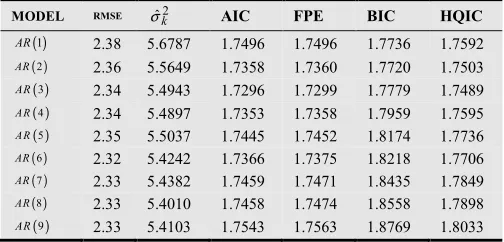
Table 4. _{LAG-SELECTION BY CONVENTIONAL INFORMATION}

CRITERIA

MODEL RMSE σˆ_k2 AIC FPE BIC HQIC ( )1

AR _2.38 _5.6787 _1.7496 _1.7496 _1.7736 _1.7592 ( )2

AR 2.36 5.5649 1.7358 1.7360 1.7720 1.7503

( )3

AR 2.34 5.4943 1.7296 1.7299 1.7779 1.7489

( )4

A R _2.34 _5.4897 _1.7353 _1.7358 _1.7959 _1.7595 ( )5

A R _2.35 _5.5037 _1.7445 _1.7452 _1.8174 _1.7736 ( )6

AR _2.32 _5.4242 _1.7366 _1.7375 _1.8218 _1.7706 ( )7

AR 2.33 5.4382 1.7459 1.7471 1.8435 1.7849

( )8

AR 2.33 5.4010 1.7458 1.7474 1.8558 1.7898

( )9

AR _2.33 _5.4103 _1.7543 _1.7563 _1.8769 _1.8033

Table 4 has autoregressive (AR) models of order 1 to 9 in the first column and root mean square error (RMSE) for each model in the second column. The optimal truncation lag for a particular criterion is the lag that minimizes the value of that criterion. Hence, the optimal truncation lag chosen by AIC, FPE and HQIC is 3 respectively whilst BIC picked 2.This is clearly an over-specification of truncation lag when compared with truncation lag suggested by our new criterion.

8. Conclusion

In this paper, we have highlighted the lag selection problem in the context of ADF and DF-GLS tests based on standard information criteria which we have shown to over-estimate the truncation lag leading to the well-known problem of low-power associated with unit root tests. Given the persistent problem of over-specification of truncation lag by data-dependent standard information criteria, we introduced a new lag selection criterion based on Koyck distributed lag model where truncation lag is specified as a deterministic function of the partial correlation coefficient between dependent variable and different choices of independent variables of distributed lag specifications of ADF and DF-GLS unit root tests. This new procedure was shown to avoid the problem of over-specification that is commonly associated with standard information criteria that are commonly used by applied researchers for lag-selection.

References

[1] Schwert, G.W. (1989) “Tests for Unit Roots: A Monte Carlo Investigation,” Journal of Business and Economic Statistics, 7, 147-160.

[2] Campbell, J. C. and Perron, P. (1991) “Pitfall and Opportunities: What Macroeconomists shouldknow about Unit Roots,” NBER Technical Working Paper # 100

[3] Xiao, Z. and Phillips, P. C. B. (1997) “An ADF Coefficient Test for a Unit Root in ARMAModels of Unknown Order with Empirical Applications to the U.S. Economy,” CowlesFoundation Discussion Paper # 1161,

[4] Maddala, G. S. and Kim, I. M. (1998) Unit Roots, Cointegration and Time Series, Cambridge University Press

[5] Cavaliere, G. (2012) “Lag-length Selection for a Unit Root test in the presence of non-stationaryVolatility,” Cowles Foundation Discussion Paper # 1844.

[6] Dufour, J. M and King, M. L. (1991) “Optimal Invariant Tests for the Autocorrelation Coefficient in Linear Regressions with Stationary or Non-stationary AR(1) errors,” Journal of Econometrics,47, 115-143

[7] Said, E. S. and Dickey, D. A. (1984) “Testing for a Unit Root in Autoregressive Moving Average Models of Unknown Order,” Biometrika, 71, 3, 599-607.

[8] Elliott, G. Rothenberg, T. J. and Stock, J. H. (1996) “Efficient Tests for an Autoregressive UnitRoot,” Econometrica, 64, 4, 813-836

[9] Hall, A. (1994) “Testing for a Unit Root in Time Series with Pretest Data-based ModelSelection,” Journal of Business and Economic Statistics, 12, 4, 461-470

[10] Ng, S. and Perron, P. (2001) “Lag Length Selection and the Construction of Unit Root Tests with Good Size and Power,” Econometrica, 69, 6, 1519-1554

[11] Shaowen Wu (2010)”Lag Length Selection In DF-GLS Unit Root Tests”,Communication in Statistics-Simulation and computation,39:8,1590-1604

[12] Akaike, H., 1969. Fitting Autoregressive Models for Prediction. Annalsof The Institute of Statistical Mathematics, 21(2), 243–247.

[13] Akaike, H., 1973. Information theory and an extension of the maximum likelihood principle. In: Petrov, B.N., Csaki, F., 2ndInternational Symposium on Information Theory. AkademiaiKiado`, Budapest, pp. 267–281.

[14] Schwarz, G. (1978) “ Estimating the dimension of a model”. Annals of Statistics, 6, 461 –464.

[15] Hannan, E. J. and Quinn, B. G. (1978). “The determination of the order of an autoregression”. Journal of Royal Statistical Society, 41, 190 – 195.

[16] Koyck, L.M. (1954), Distributed Lags and Investment Analysis, Amsterdam: North-Holland.