Active Learning in Approximately Linear Regression
Based on Conditional Expectation of Generalization Error
Masashi Sugiyama [email protected]
Department of Computer Science Tokyo Institute of Technology
2-12-1, O-okayama, Meguro-ku, Tokyo, 152-8552, Japan
Editor: Greg Ridgeway
Abstract
The goal of active learning is to determine the locations of training input points so that the general-ization error is minimized. We discuss the problem of active learning in linear regression scenarios. Traditional active learning methods using least-squares learning often assume that the model used for learning is correctly specified. In many practical situations, however, this assumption may not be fulfilled. Recently, active learning methods using “importance”-weighted least-squares learning have been proposed, which are shown to be robust against misspecification of models. In this paper, we propose a new active learning method also using the weighted least-squares learning, which we call ALICE (Active Learning using the Importance-weighted least-squares learning based on Con-ditional Expectation of the generalization error). An important difference from existing methods is that we predict the conditional expectation of the generalization error given training input points, while existing methods predict the full expectation of the generalization error. Due to this dif-ference, the training input design can be fine-tuned depending on the realization of training input points. Theoretically, we prove that the proposed active learning criterion is a more accurate pre-dictor of the single-trial generalization error than the existing criterion. Numerical studies with toy and benchmark data sets show that the proposed method compares favorably to existing methods.
Keywords: Active Learning, Conditional Expectation of Generalization Error, Misspecification
of Models, Importance-Weighted Least-Squares Learning, Covariate Shift.
1. Introduction
In a standard setting of supervised learning, the training input points are provided from the envi-ronment (Vapnik, 1998). On the other hand, there are cases where the location of the training input points can be designed by users (Fedorov, 1972; Pukelsheim, 1993). In such situations, it is expected that the accuracy of learned results can be improved by appropriately choosing the location of the training input points, e.g., by densely allocating the training input points in the regions with high un-certainty. Active learning (MacKay, 1992; Cohn et al., 1996; Fukumizu, 2000)—also referred to as
experimental design in statistics (Kiefer, 1959; Fedorov, 1972; Pukelsheim, 1993)—is the problem
of optimizing location of training input points so that the generalization error is minimized.
with OLS tries to determine the location of the training input points so that the variance term is minimized (Fedorov, 1972). In practice, however, the correctness of the model may not be fulfilled. Active learning is a situation under the covariate shift (Shimodaira, 2000), where the training input distribution is different from the test input distribution. When the model used for learning is correctly specified, the covariate shift does not matter because OLS is still unbiased under a mild condition. However, OLS is no longer unbiased even asymptotically for misspecified models, and therefore we have to explicitly deal with the bias term if OLS is used.
Under the covariate shift, it is known that a form of weighted least-squares learning (WLS) is shown to be asymptotically unbiased even for misspecified models (Shimodaira, 2000; Wiens, 2000). The key idea of this WLS is the use of the ratio of density functions of test and training input points: the goodness-of-fit of the training input points is adjusted to that of the test input points by the density ratio, which is similar to importance sampling.
In this paper, we propose a variance-only active learning method using WLS, which can be regarded as an extension of the traditional variance-only active learning method using OLS. The proposed method can be theoretically justified for the approximately correct models, and thus is
robust against the misspecification of models.
Conditional Expectation of Generalization Error: A variance-only active learning method us-ing WLS has also been proposed by Wiens (2000), which can also be theoretically justified for ap-proximately correct models. The important difference is how the generalization error is predicted: we predict the conditional expectation of the generalization error given training input points, while in Wiens (2000), the full expectation of the generalization error is predicted. In order to explain this difference in more detail, we first note that the generalization error of the WLS estimator depends on the training input density since WLS explicitly uses it. Therefore, when WLS is used in active learning, the generalization error is predicted as a function of the training input density, and the training input density is optimized so that the predicted generalization error is minimized.
The parameters in the model are learned using the training examples, which consist of training input points drawn from the user-designed distribution and corresponding noisy output values. This means that the generalization error is a random variable which depends on the location of the train-ing input points and noise contained in the traintrain-ing output values. We ideally want to predict the
single-trial generalization error, i.e., the generalization error for a single realization of the training
examples at hand. From this viewpoint, we do not want to average out the random variables, but we want to plug the realization of the random variables into the generalization error and evaluate the realized value of the generalization error. However, we may not be able to avoid taking the expec-tation over the training output noise since the training output noise is inaccessible. In contrast, the location of the training input points are accessible by nature. Motivated by this fact, in this paper, we predict the generalization error without taking the expectation over the training input points. That is, we predict the conditional expectation of the generalization error given training input points. On the other hand, in Wiens (2000), the generalization error is predicted in terms of the expectation over both the training input points and the training output noise.
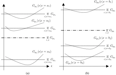
A possible advantage of the conditional-expectation approach is schematically illustrated in Figure 1. For illustration purposes, we consider the case of sampling only one training example. The solid curves in the left graph (Figure 1-(a)) depict Gpa(ε|x), the generalization error for a training input density paas a function of the training output noiseεgiven a training input point x. The three
(a) (b)
Figure 1: Schematic illustration of conditional expectation and full expectation of the generaliza-tion error. (a) and (b) correspond to the generalizageneraliza-tion error for paand pb, respectively.
and a3, respectively. The value of the generalization error for the density pain the full-expectation
approach is depicted by the dash-dotted line, where the generalization error is expected over both the training output noiseεand the training input points x (i.e., the mean of the three solid curves). The values of the generalization error in the conditional-expectation approach are depicted by the dotted lines, where the generalization errors are expected only over the training output noiseε, given
x=a1,a2,a3, respectively (i.e., the mean of each solid curve). The right graph (Figure 1-(b)) depicts the generalization errors for the training input density pbin the same manner.
In the full-expectation framework, the density pais judged to be better than pbregardless of the
realization of the training input point since the dash-dotted line in the left graph is lower than that in the right graph (see Figure 1 again). However, as the solid curves show, pais often worse than pb
in single trials. On the other hand, in the conditional-expectation framework, the goodness of the density is adaptively judged depending on the realizations of the training input point x. For example,
pb is judged to be better than paif a2and b3are realized, or pais judged to be better than pb if a3
and b1are realized. That is, the conditional-expectation framework may yield a better choice of the training input density (and the training input points) than the full-expectation framework.
proposed method compares favorably to Wiens’s method in the simulations with toy and benchmark data sets.
Bias-and-Variance Approach for Misspecified Models: Kanamori and Shimodaira (2003) also proposed an active learning algorithm using WLS. This method is not variance-only, but it takes both the bias and the variance into account by gathering training input points in two stages. In the first stage, a certain number of training examples are randomly gathered from the environment, and the generalization error (i.e., the sum of the bias and variance) is predicted by using the gathered training examples. Then in the second stage, the training input density for the remaining training examples is optimized based on the generalization error prediction. Theoretically, the two-stage method is shown to asymptotically give the optimal training input density not only for approximately correct models, but also for totally misspecified models. Although this property is solid, it may not be practically valuable since learning with totally misspecified models may not work well because of the model error. A drawback of this method is that it requires some randomly collected training examples in the first stage, so we are not allowed to optimally design all the training input locations by ourselves. Our experiments show that the proposed method works better than the two-stage method of Kanamori and Shimodaira (2003).
Batch Selection of Training Input Points: Active learning in the machine learning community is often thought of as being a sequential process: selecting one or a few training input points, observing corresponding training output values, training the model using the gathered training examples, and iterating this process. An alternative approach is the batch approach, where all training input points are gathered in the beginning.
If the environment is non-stationary, i.e., the learning target function drifts, taking the sequential approach would be necessary. On the other hand, under the stationary environment, i.e., the learning target function is fixed, the batch approach gives the globally optimal solution and the sequential approach can be regarded as a greedy approximation to it. In this paper, we consider the stationary case, so the batch approach is desirable.
In correctly specified linear regression, the expected generalization error does not depend on the learning target function under a mild condition. Therefore, the globally optimal solution can be obtained in principle. However, in misspecified linear regression which we discuss in this paper, the expected generalization error depends on the unknown learning target function. In this scenario, the sequential approach would be natural: estimating the unknown learning target function and optimizing location of the training input points are carried out alternately. On the other hand, in this paper, we do not estimate the learning target function, but we approximate the generalization error by the quantity which does not depend on the learning target function. This makes it possible to take the batch approach of determining all the training input points at once in advance.
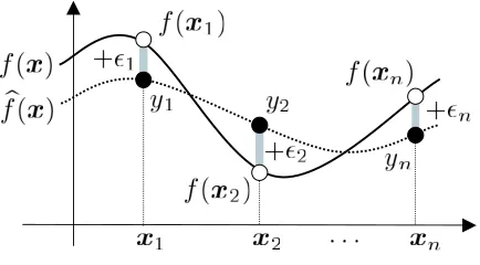
Figure 2: Regression problem.
seems to be a popular approach in batch active learning research (Wiens, 2000; Kanamori and Shimodaira, 2003).
Organization: The rest of this paper is organized as follows. We derive a new active learning method in Section 2, and we discuss relations between the proposed method and the existing meth-ods in Section 3. We report numerical results using toy and benchmark data sets in Section 4. Finally, we state conclusions and future prospects in Section 5.
2. Derivation of New Active Learning Method
In this section, we formulate the active learning problem in regression scenarios, and derive a new active learning method.
2.1 Problem Formulation
Let us discuss the regression problem of learning a real-valued function f(x)defined onRd from training examples (see Figure 2). Training examples are given as
{(xi,yi)|yi=f(xi) +εi}ni=1,
where{εi}ni=1are i.i.d. noise with mean zero and unknown varianceσ2. We suppose that the training input points{xi}n
i=1are independently drawn from a user-defined distribution with density p(x). Let bf(x) be a learned function obtained from the training examples{(xi,yi)}n
i=1. We evaluate the goodness of the learned function bf(x)by the expected squared test error over test input points, to which refer as the generalization error. When the test input points are drawn independently from a distribution with density q(x), the generalization error G0is expressed as
G0=
Z
b
f(x)−f(x)2q(x)dx. (1) We suppose that q(x)is known (or its reasonable estimate is available). This seems to be a com-mon assumption in active learning literature (e.g., Fukumizu, 2000; Wiens, 2000; Kanamori and Shimodaira, 2003). If a large number of unlabeled samples1are easily gathered, a reasonably good
estimate of q(x) may be obtained by some standard density estimation method. Therefore, the assumption that q(x)is known or its reasonable estimate is available may not be so restrictive.
In the following, we discuss the problem of optimizing the training input density p(x) so that the generalization error is minimized.
2.2 Approximately Correct Linear Regression
We learn the target function f(x)by the following linear regression model:
b f(x) =
b
∑
i=1
b
αiϕi(x), (2)
where{ϕi(x)}bi=1are fixed linearly independent functions2andαb= (α1,b bα2, . . . ,αbb)>are parameters
to be learned (by a variant of least-squares, see Section 2.4 for detail).
Suppose the regression model (2) does not exactly include the learning target function f(x), but it approximately includes it, i.e., for a scalarδsuch that|δ|is small, f(x)is expressed as
f(x) =g(x) +δr(x), (3)
where g(x)is the optimal approximation to f(x)by the model (2):
g(x) =
b
∑
i=1 α∗
iϕi(x).
α∗= (α∗
1,α∗2, . . . ,α∗b)>is the unknown optimal parameter defined by
α∗=argmin α
Z b
∑
i=1
αiϕi(x)−f(x) !2
q(x)dx.
δr(x)in Eq.(3) is the residual, which is orthogonal to{ϕi(x)}bi=1under q(x)(see Figure 3):
Z
r(x)ϕi(x)q(x)dx=0 for i=1,2, . . . ,b. (4)
The function r(x)governs the nature of the model error, andδis the possible magnitude of this error. In order to separate these two factors, we further impose the following normalization condition on
r(x):
Z
r2(x)q(x)dx=1. (5)
Note that we are essentially estimating the projection g(x), rather than the true target function f(x).
Figure 3: Orthogonal decomposition of f(x).
2.3 Bias/Variance Decomposition of Generalization Error
As described in Section 1, we evaluate the generalization error in terms of the expectation over only the training output noise{εi}ni=1, not over the training input points{xi}ni=1.
LetE{εi}denote the expectation over the noise{εi}ni=1. Then, the generalization error expected over the training output noise can be decomposed into the (squared) bias term B, the variance term
V , and the model error C:
E {εi}
G0=B+V+C,
where
B=
Z
E {εi}
b
f(x)−g(x)
!2
q(x)dx,
V = E {εi}
Z
b
f(x)− E {εi}
b f(x)
!2
q(x)dx,
C=
Z
(g(x)−f(x))2q(x)dx. (6) Since C is constant which depends neither on p(x)nor{xi}ni=1, we subtract C from G0and define it by G.
G=G0−C.
2.4 Importance-Weighted Least-Squares Learning
Let X be the design matrix, i.e., X is the n×b matrix with the(i,j)-th element
Xi,j=ϕj(xi).
A standard way to learn the parameters in the regression model (2) is the ordinary least-squares
(OLS) learning, i.e., parameter vectorαis determined as follows.
b
αO=argmin
α
" n
∑
i=1
b f(xi)−yi
2#
, (7)
where the subscript ‘O’ indicates the ordinary LS.αbOis analytically given by b
where
LO= (X>X)−1X>,
y= (y1,y2, . . . ,yn)>.
When the training input points{xi}ni=1are drawn from q(x), OLS is asymptotically unbiased even for misspecified models. However, the current situation is under the covariate shift (Shimodaira, 2000), where the training input density p(x)is generally different from the test input density q(x). Under the covariate shift, OLS is no longer unbiased even asymptotically for misspecified models. On the other hand, it is known that the following weighted least-squares (WLS) learning is asymptotically unbiased (Shimodaira, 2000).
b
αW =argmin
α
" n
∑
i=1
q(xi)
p(xi)
b f(xi)−yi
2#
, (8)
where the subscript ‘W ’ indicates the weighted LS. Asymptotic unbiasedness ofbαW would be
intu-itively understood by the following identity, which resembles the importance sampling:
Z
b
f(x)−f(x)2q(x)dx=
Z
b
f(x)−f(x)2q(x)
p(x)p(x)dx.
In the following, we assume that p(x)and q(x)are strictly positive for all x. Let D be the diagonal matrix with the i-th diagonal element
Di,i= q(xi) p(xi)
.
ThenbαW is analytically given by
b
αW=LWy, (9)
where
LW = (X>DX)−1X>D.
2.5 Active Learning Based on Importance-Weighted Least-Squares Learning
Let GW, BW and VW be G, B and V for the learned function obtained by WLS, respectively. Let U
be the b-dimensional square matrix with the(i,j)-th element
Ui,j=
Z
ϕi(x)ϕj(x)q(x)dx.
Then we have the following lemma (Proofs of all lemmas are provided in appendices). Lemma 1 For the approximately correct model (3), we have
BW =
O
p(δ2n−1), (10)Input: A finite set
P
b of strictly positive probability densitiesCalculate U . For each p∈
P
bCreate training input points{x(ip)}ni=1following p(x). Calculate LW.
Calculate J(p). End
Choose bp that minimizes J.
Put xi=x(ipb)for i=1,2, . . . ,n.
Observe the training output values{yi}ni=1at{xi}ni=1. CalculateαbW by Eq.(9).
Output: bαW
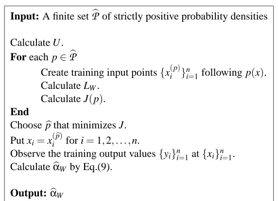
Figure 4: Proposed ALICE algorithm.
Note that the asymptotic order in the above lemma is in probability since random variables
{xi}ni=1are included. This lemma implies that ifδ=op(1), E
{εi}
GW =σ2tr(U LWL>
W) +op(n−1). (11)
Motivated by Eq.(11), we propose determining the training input density p(x)as follows: For a set
P
of strictly positive probability densities,p∗=argmin
p∈P
J(p),
where
J=tr(U LWL>W). (12)
Practically, we may prepare a finite set
P
b of strictly positive probability densities and choose theone that minimizes J from the set
P
b. A pseudo code of the proposed active learning algorithm isdescribed in Figure 4, which we call ALICE (Active Learning using the Importance-weighted least-squares learning based on Conditional Expectation of the generalization error). Note that the value of J depends not only on p(x), but also on the realization of the training input points{x(ip)}ni=1.
3. Relation to Existing Methods
In this section, we qualitatively compare the proposed active learning method with existing methods. 3.1 Active Learning with OLS
Let GO, BOand VObe G, B and V for the learned function obtained by OLS, respectively. Ifδ=0
in Eq.(3), i.e., the model is correctly specified, BOvanishes under a mild condition (Fedorov, 1972)
and we have
E {εi}
GO=VO=σ2tr(U LOL>
Based on the above expression, the training input density p(x) is determined3 as follows (Fe-dorov, 1972; Cohn et al., 1996; Fukumizu, 2000).
p∗O=argmin
p∈P
JO(p),
where
JO=tr(U LOL>O). (13)
Comparison with J: We investigate the validity of JOfor approximately correct models based on
the following lemma.
Lemma 2 For the approximately correct model (3), we have
BO=
O
(δ2),VO=
O
p(n−1).The above lemma implies that ifδ=op(n−
1 2),
E {εi}
GO=σ2JO+op(n−1).
Therefore, if δ=op(n−12), the use of JO can be still justified. On the other hand, the proposed
J is valid when δ=op(1). This implies that J has a wider range of applications than JO. As
experimentally shown in Section 4, this difference is highly significant in practice. 3.2 Active Learning with WLS: Variance-Only Approach
For the importance-weighted least-squares learning (8), Kanamori and Shimodaira (2003) proved that the generalization error expected over training input points{xi}ni=1 and training output noise
{εi}ni=1is asymptotically expressed as
E {xi}
E {εi}
GW =1
ntr(U
−1H) +
O
(n−32), (14)
whereE{xi}is the expectation over training input points{xi}
n
i=1and H is the b-dimensional square matrix defined by
H=S+σ2T.
S and T are the b-dimensional square matrices with the(i,j)-th elements
Si,j=
Z
ϕi(x)ϕj(x)(δr(x))2 q(x)2
p(x)dx, (15)
Ti,j=
Z
ϕi(x)ϕj(x) q(x)2
p(x)dx.
(16)
3. p(x)is not explicitly used in OLS. Therefore, we do not have to optimize the training input density p(x), but we can directly optimize training input points{xi}ni=1. However, to be consistent with the WLS-based methods, we optimize
Note that 1ntr(U−1S)corresponds to the squared bias while σn2tr(U−1T)corresponds to the variance. Eq.(14) suggests that tr(U−1H)may be used as an active learning criterion. However, H includes the inaccessible quantitiesδr(x)andσ2, so tr(U−1H)can not be directly calculated.
To cope with this problem, Wiens (2000) proposed4ignoring S (the bias term), which yields
E {xi}
E {εi}
GW ≈σ
2
n tr(U
−1T).
Note that T is accessible under the current setting. Based on this approximation, the training input density p(x)is determined as follows.
p∗W =argmin
p∈P
JW(p),
where
JW =1
ntr(U
−1T). (17)
Comparison with J: A notable feature of JW is that the optimal training input density pW∗(x)can
be obtained analytically (Wiens, 2000):
pW∗(x) = bh(x)
Rb
h(x)dx, (18)
where
bh(x) =q(x)
b
∑
i,j=1
Ui−,j1ϕi(x)ϕj(x) !1
2 .
This may be confirmed by the fact that JW can be expressed as
JW(p) =
1
n Z
b h(x)dx
2 1+
Z (p∗
W(x)−p(x))2 p(x) dx
.
On the other hand, we do not yet have an analytic form of a minimizer for the criterion J.
It seems that in Wiens (2000), ignoring S has not been well justified. Here, we investigate the validity based on the following corollary immediately obtained from Eqs.(14) and (15).
Corollary 1 For the approximately correct model (3), we have
E {xi}
E {εi}
GW =σ2JW+
O
(δ2n−1+n−3 2),
whereσ2JW =
O
(n−1).This corollary implies that ifδ=o(1), E {xi}
E {εi}
GW =σ2JW+o(n−1),
by which the use of JW can be justified asymptotically. Since the order is the same as that of the
proposed criterion, J and JW may be comparable in the robustness against the misspecification of
models.
Now the following lemma reveals a more direct relation between J and JW.
Lemma 3 J and JW satisfy
J=JW+
O
p(n−3
2). (19)
This lemma implies that J is asymptotically equivalent to JW. However, they are still different
in the order of n−1. In the following, we show that this difference is important.
In the active learning context, we are interested in accurately predicting the single-trial gener-alization error GW, which depends on the realization of the training examples. Let us measure the
goodness of a generalization error predictorG byb
E {εi}
(Gb−GW)2. (20)
Then we have the following lemma. Lemma 4 Supposeδ=op(n−
1
4). If terms of op(n−3)are ignored, we have E
{εi} (σ2J
W−GW)2≥ E
{εi}
(σ2J−G
W)2.
This lemma states that underδ=op(n−
1
4),σ2J is asymptotically a more accurate estimator of the single-trial generalization error GW thanσ2JW in the sense of Eq.(20).
In Section 4, we experimentally evaluate the difference between J and JW.
3.3 Active Learning with WLS: Bias-and-Variance Approach
Another idea of approximating H in Eq.(14) is a two-stage sampling scheme proposed5by Kanamori and Shimodaira (2003): the training examples sampled in the first stage are used for estimating H and in the second stage, the distribution of the remaining training input points is optimized based on the estimated H. We explain the details of the algorithm below.
First, ` (≤n) training input points {exi}`i=1 are created independently following the test input distribution with density q(x), and corresponding training output values{yie}`i=1 are observed. Let
e
D andQ be thee `-dimensional diagonal matrices with the i-th diagonal elements
e Di,i=
q(exi) p(exi),
e
Qi,i= [ey−Xe(Xe>Xe)−1Xe>ey]i,
where [·]i denotes the i-th element of a vector. X is the design matrix fore {exi}`i=1, i.e., the `×b matrix with the(i,j)-th element
e
Xi,j=ϕj(exi),
and
ey= (ey1,ye2, . . . ,ey`)>.
Then an approximationH of the unknown matrix H in Eq.(14) is given bye e
H=1 `Xe
>e
DQe2Xe.
Although U−1is accessible in the current setting, Kanamori and Shimodaira (2003) also replaced it by a consistent estimateUe−1, where
e U=1
`Xe >e
X.
Based on the above approximations, the training input density p(x)is determined as follows:
p∗OW =argmin
p∈P
JOW(p),
where
JOW =
1
ntr(Ue
−1
e
H). (21)
Note that the subscript ‘OW ’ indicates the combination of the ordinary LS and weighted LS (see below for details).
After determining the optimal density p∗OW, the remaining n−`training input points {xi}ni=−1`
are created independently following p∗OW(x), and corresponding training output values{yi}ni=−1`are observed. Then the learned parameterbαOW is obtained using{(exi,eyi)}`i=1and{(xi,yi)}ni=−1`as
b
αOW =argmin
α
"
`
∑
i=1
b f(exi)−eyi
2 +
n−`
∑
i=1
q(xi) p(xi)
b f(xi)−yi
2#
. (22)
Note that JOW depends on the realization of{exi}`i=1, but is independent of the realization of{xi}ni=−1`. Comparison with J: Kanamori and Shimodaira (2003) proved that for`=o(n), limn→∞`=∞, andδ=
O
(1),E {xi}
E {εi}
GW =1
nJOW+o(n
−1),
by which the use of JOW can be justified. The order ofδrequired above is weaker than that required
in J. Therefore, JOW may have a wider range of applications than J. However, this property may
not be practically valuable since learning with totally misspecified models (i.e.,δ=
O
(1)) may notwork well because of the model error.
Shimodaira (2003), but the exact choice of`seems still open. Third, JOW is an estimator of GW, but
the finally obtained parameter by this algorithm is notbαW butαbOW. Therefore, this difference can
degrade the performance.6
In Section 4, we experimentally compare J and JOW.
4. Numerical Examples
In this section, we quantitatively compare the proposed and existing active learning methods through numerical experiments.
4.1 Toy Data Set
We first illustrate how the proposed and existing methods behave under a controlled setting. Setting: Let the input dimension be d=1 and the learning target function be
f(x) =1−x+x2+δr(x), where
r(x) =z 3−3z
√
6 with z=
x−0.2
0.4 . (23)
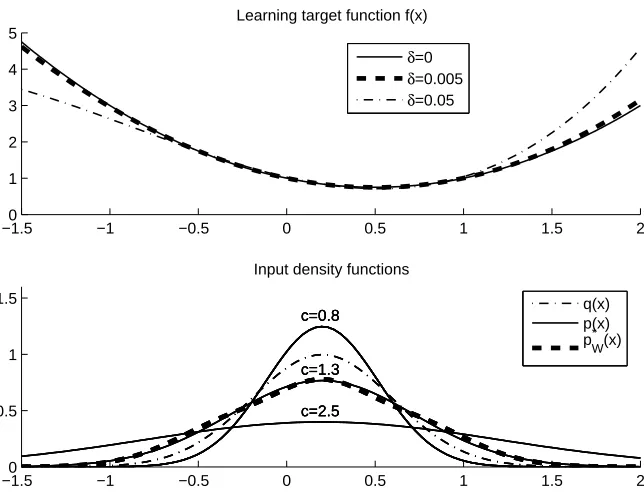
Let the number of training examples to gather be n=100 and{εi}ni=1be i.i.d. Gaussian noise with mean zero and standard deviation 0.3. Let the test input density q(x)be the Gaussian density with mean 0.2 and standard deviation 0.4, which is assumed to be known in this illustrative simulation. See the bottom graph of Figure 5 for the profile of q(x). Let the number of basis functions be b=3 and the basis functions be
ϕi(x) =xi−1 for i=1,2, . . . ,b.
Note that for these basis functions, the residual function r(x)in Eq.(23) fulfills Eqs.(4) and (5). Let us consider the following three cases.
δ=0,0.005,0.05, (24)
which correspond to “correctly specified”, “approximately correct”, and “misspecified” cases, re-spectively. See the top graph of Figure 5 for the profiles of f(x)with differentδ.
As a set of training input densities,
P
b, we use the Gaussian densities with mean 0.2 and standarddeviation 0.4c, where
c=0.8,0.9,1.0, . . . ,2.5.
See the bottom graph of Figure 5 again for the profiles of p(x)with different c. In this experiment, we compare the performance of the following methods:
(ALICE): c is determined so that J given by Eq.(12) is minimized. WLS given by Eq.(8) is used for estimating the parameters.
6. It is possible to resolve this problem by not using{(exi,yei)}`i=1gathered in the first stage for estimating the parameter
−1.50 −1 −0.5 0 0.5 1 1.5 2 1
2 3 4 5
Learning target function f(x)
−1.50 −1 −0.5 0 0.5 1 1.5 2
0.5 1 1.5
c=0.8
c=1.3
c=2.5 c=0.8
c=1.3
c=2.5 c=0.8
c=1.3
c=2.5
Input density functions
δ=0
δ=0.005
δ=0.05
q(x) p(x) p
W *(x)
Figure 5: Learning target function and input density functions.
(W): c is determined so that JW given by Eq.(17) is minimized. WLS is used for estimating the
parameters.
(W*): p∗W(x)given by Eq.(18) is used as the training input density. The profile of pW∗ (x)under the current setting is illustrated in the bottom graph of Figure 5, showing that pW∗ (x)is similar to the Gaussian density with c=1.3. WLS is used for estimating the parameters.
(OW): First, ` training input points are created following the test input density q(x), and corre-sponding training output values are observed. Based on the`training examples, c is deter-mined so that JOW given by Eq.(21) is minimized. Then n−`remaining training input points
are created following the determined input density. The combination of OLS and WLS given by Eq.(22) is used for estimating the parameters. We set`=25, which we experimentally confirmed to be a reasonable choice in this illustrative simulation.
(O): c is determined so that JO given by Eq.(13) is minimized. OLS given by Eq.(7) is used for
estimating the parameters.
(Passive): Following the test input density q(x), training input points{xi}ni=1 are created. OLS is used for estimating the parameters.
For (W*), we generate the random number following p∗W(x)by the rejection method (see e.g., Knuth, 1998). We run this simulation 1000 times for eachδin Eq.(24).
Accuracy of Generalization Error Prediction: First, we evaluate the accuracy of J, JW, JOW,
and JOas predictors of the generalization error. Note that J and JW are predictors of GW. JOW is also
δ=0 δ=0.005 δ=0.05 “correctly specified” “approximately correct” “misspecified”
0.8 1.2 1.6 2 2.4 0 0.002 0.004 0.006 0.008 0.01 GW
0.8 1.2 1.6 2 2.4 0 0.002 0.004 0.006 0.008 0.01 J
0.8 1.2 1.6 2 2.4 0 0.002 0.004 0.006 0.008 0.01 JW
0.8 1.2 1.6 2 2.4 0 0.002 0.004 0.006 0.008 0.01 GOW
0.8 1.2 1.6 2 2.4 0 0.002 0.004 0.006 0.008 0.01 J OW
0.8 1.2 1.6 2 2.4 0 0.002 0.004 0.006 0.008 0.01 G O
0.8 1.2 1.6 2 2.4 0 0.002 0.004 0.006 0.008 0.01 c J O
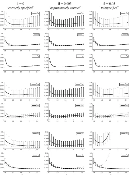
Figure 6: The means and (asymmetric) standard deviations of GW, J, JW, GOW, JOW, GO, and JO
is the generalization error G for the learned function obtained by the combination of OLS and WLS (see Eq.(22)). Therefore, JOW should be evaluated as a predictor of GOW. JOis a predictor of GO.
In Figure 6, the means and standard deviations of GW, J, JW, GOW, JOW, GO, and JOover 1000
runs are depicted as functions of c by the solid curves. Here the upper and lower error bars are calculated separately since the distribution is not symmetric. The dashed curves show the means of the generalization error that corresponding active learning criteria are trying to predict. Note that
J, JW, and JO are multiplied by σ2= (0.3)2 so that comparison with GW and GO are clear. By
definition, GW, GOW, and GOdo not include the constant C defined by Eq.(6). The values of C for
δ=0, 0.005, and 0.05 are 0, 2.32×10⁻⁵, and 2.32×10⁻³, respectively.
These graphs show that whenδ=0 (“correctly specified”), J and JW give accurate predictions
of GW. Note that JW does not depend on the training input points{xi}ni=1 so it does not fluctuate
over 1000 runs. JOW is slightly biased toward the negative direction for small c. We conjecture that
this is caused by the small sample effect. However, the profile of JOW still roughly approximates
that of GOW. JO gives accurate predictions of GO. Whenδ=0.005 (“approximately correct”), J, JW, and JOW work similarly to the case withδ=0, i.e., J and JW are accurate and JOW is negatively
biased. On the other hand, JObehaves slightly differently: it tends to be biased toward the negative
direction for large c. Finally, whenδ=0.05 (“misspecified”), J and JW still give accurate
predic-tions, although they slightly have a negative bias for small c. JOW still roughly approximates GOW,
while JOgives totally different profile from GO.
These results show that as approximations of the generalization error, J and JW are accurate and
robust against the misspecification of models. JOW is also reasonably accurate, although it tends to
be rather inaccurate for small c. JOis accurate in the correctly specified case, but it becomes totally
inaccurate once the correctness of the model is violated.
Note that, by definition, J, JW and JOdo not depend on the learning target function. Therefore,
in the simulation, they give the same values for allδ(J and JOdepend on the realization of{xi}ni=1so they may have a small fluctuation). On the other hand, the generalization error, of course, depends on the learning target function even if the constant C is not included, since the training output values depend on it. Note that the bias depends onδ, but the variance does not. The simulation results show that the profile of GOchanges heavily as the degree of model misspecification increases. This would
be caused by the increase of the bias since OLS is not unbiased even asymptotically. On the other hand, JO stays the same asδincreases. As a result, JObecomes a very poor predictor for a large
δ. In contrast, the profile of GW appears to be very stable against the change inδ, which is in good
agreement with the theoretical fact that WLS is asymptotically unbiased. Thanks to this property, J and JW are more accurate than JOfor misspecified models.
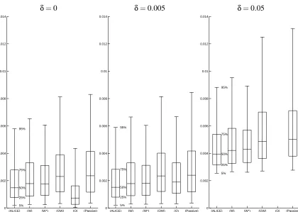
Obtained Generalization Error: In Table 1, the mean and standard deviation of the generaliza-tion error obtained by each method are described. The best method and comparable ones by the
t-test (e.g., Henkel, 1979) at the significance level 5% are indicated with boldface. In Figure 7, the
box-plot expression of the obtained generalization error is depicted. Note that the values described in Figure 6 correspond to G (the constant C is not included), while the values in Table 1 and Figure 7 correspond to G0 which includes C (see Eq.(1)).
Whenδ=0, (O) works significantly better than other methods. Actually, in this case, training input densities that approximately minimize GW, GO, and GOW were successfully found by
δ=0 δ=0.005 δ=0.05 (ALICE) 2.08±1.95 2.10±1.96 4.61±2.12
(W) 2.40±2.15 2.43±2.15 4.89±2.26 (W*) 2.32±2.02 2.35±2.02 4.84±2.14 (OW) 3.09±3.03 3.13±3.00 5.95±3.58 (O) 1.31±1.70 2.53±2.23 124±67.4 (Passive) 3.11±2.78 3.14±2.78 6.01±3.43
All values in the table are multiplied by 103.
Table 1: The mean and standard deviation of the generalization error obtained by each method for the toy data set. Here we describe the value G0 that includes the constant C (see Eq.(6)). The best method and comparable ones by the t-test at the significance level 5% are in-dicated with boldface. The value of (O) for δ=0.05 is extremely large but it is not a typo.
δ=0 δ=0.005 δ=0.05
(ALICE) (W) (W*) (OW) (O) (Passive) 0
0.002 0.004 0.006 0.008 0.01 0.012 0.014
5% 25% 50% 75% 95%
(ALICE) (W) (W*) (OW) (O) (Passive) 0
0.002 0.004 0.006 0.008 0.01 0.012 0.014
5% 25% 50% 75% 95%
(ALICE) (W) (W*) (OW) (O) (Passive) 0
0.002 0.004 0.006 0.008 0.01 0.012 0.014
5% 25% 50% 75% 95%
larger variance than OLS (Shimodaira, 2000). Therefore, whenδ=0, OLS would be more accurate than WLS since both WLS and OLS are unbiased. Although (ALICE), (W), (W*), and (OW) are outperformed by (O), they still work better than (Passive). Note that (ALICE) is significantly better than (W), (W*), (OW), and (Passive) by the t-test. The box-plot shows that (ALICE) outperforms (W), (W*), and (OW) particularly in upper quantiles.
Whenδ=0.005, (ALICE) gives significantly smaller errors than other methods. All the meth-ods except (O) work similarly to the case withδ=0, while (O) tends to perform poorly. This result is surprising since the learning target functions withδ=0 and δ=0.005 are visually almost the same, as illustrated in the top graph of Figure 5. Therefore, it intuitively seems that the result when δ=0.005 is not much different from the result whenδ=0. However, this slight difference appears to make (O) unreliable.
Whenδ=0.05, (ALICE) again works significantly better than others. (W) and (W*) still work reasonably well. The box-plot shows that (ALICE) is better than (W) and (W*) particularly in upper quantiles. The performance of (OW) is slightly degraded, although it is still better than (Passive). (O) gives extremely large errors.
The above results are summarized as follows. For all three cases (δ=0,0.005,0.05), (ALICE), (W), (W*), and (OW) work reasonably well and consistently outperform (Passive). Among them, (ALICE) appears to be better than (W), (W*), and (OW) for all three cases. (O) works excellently in the correctly specified case, although it tends to perform poorly once the correctness of the model is violated. Therefore, (ALICE) is found to work well overall and is robust against the misspecification of models for this toy data set.
4.2 Benchmark Data Sets
Here we use eight regression benchmark data sets provided by DELVE (Rasmussen et al., 1996):
Bank-8fm, Bank-8fh, Bank-8nm, Bank-8nh, Kin-8fm, Kin-8fh, Kin-8nm, and Kin-8nh. Each data set
includes 8192 samples, consisting of 8-dimensional input points and 1-dimensional output values. For convenience, every attribute is normalized into[0,1].
Suppose we are given all 8192 input points (i.e., unlabeled samples). Note that output values are kept unknown at this point. From this pool of unlabeled samples, we choose n=300 input points
{xi}ni=1 for training and observe the corresponding output values{yi}ni=1. The task is to predict the output values of all 8192 unlabeled samples.
In this experiment, the test input density q(x)is unknown. So we estimate it using the uncorre-lated multi-dimensional Gaussian density:
q(x) = 1 (2πbγ2
MLE)
d
2 exp
−kx−bµMLEk
2 2bγ2
MLE
,
wherebµMLE andbγMLE are the maximum likelihood estimates of the mean and standard deviation
obtained from all 8192 unlabeled samples. Let b=50 and the basis functions be Gaussian basis functions with variance 1:
ϕi(x) =exp
−kx−tik
2 2
for i=1,2, . . . ,b,
Bank-8fm Bank-8fh Bank-8nm Bank-8nh (ALICE) 2.10±0.17 6.83±0.44 1.11±0.09 4.19±0.29
(W) 2.26±0.21 7.21±0.52 1.22±0.12 4.40±0.38 (OW) 2.31±0.25 7.39±0.63 1.25±0.15 4.52±0.39 (O) 1.91±0.16 6.20±0.24 1.32±0.14 4.02±0.21 (Passive) 2.31±0.26 7.45±0.61 1.26±0.14 4.51±0.38 Kin-8fm Kin-8fh Kin-8nm Kin-8nh (ALICE) 1.62±0.58 3.50±0.63 34.97±1.90 47.21±1.97
(W) 1.70±0.62 3.64±0.73 36.60±2.05 49.15±2.88 (OW) 1.73±0.63 3.73±0.78 37.29±2.94 49.64±3.11 (O) 3.03±1.60 4.85±1.96 38.65±3.09 48.86±2.66 (Passive) 1.77±0.68 3.73±0.79 37.38±3.05 49.69±3.06
All values in the table are multiplied by 103.
Table 2: The means and standard deviations of the test error for DELVE data sets. The best method and comparable ones by the t-test at the significance level 5% are indicated with boldface.
Bank−8fm Bank−8fh Bank−8nm Bank−8nh Kin−8fm Kin−8fh Kin−8nm Kin−8nh 0.85
0.9 0.95 1 1.05 1.1
(ALICE) (W) (OW) (O) (Passive)
We select the training input density p(x)from the set of uncorrelated multi-dimensional Gaus-sian densities with meanbµMLE and standard deviation cbγMLE, where
c=0.7,0.75,0.8, . . . ,2.4.
We again compare the active learning methods tested in Section 4.1. However, we do not test (W*) here because we could not efficiently generate random numbers following pW∗(x)by the rejection method. For (OW), we set`=100 which we experimentally confirmed to be reasonable.
In this simulation, we can not create the training input points in an arbitrary location because we only have 8192 samples in the pool. Here, we first create provisional input points following the determined training input density, and then choose the input points from the pool of unlabeled samples that are closest to the provisional input points. In this simulation, the expectation over the test input density q(x)in the matrix U is calculated by the empirical average over all 8192 unlabeled samples since the true test error is also calculated as such. For each data set, we run this simulation 100 times, by changing the template points{ti}bi=1in each run.
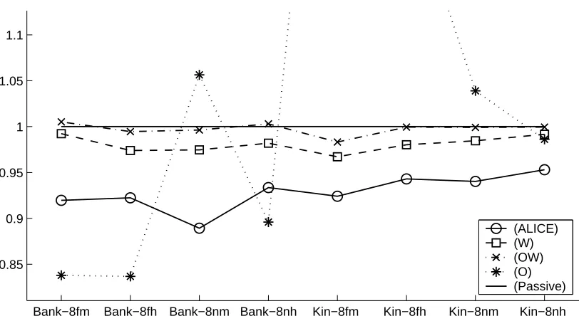
The means and standard deviations of the test error over 100 runs are described in Table 2. This shows that (ALICE) works very well for five out of eight data sets. For the other three data sets, (O) works significantly better than other methods. (W) works well and is comparable to (ALICE) for two data sets, but is outperformed by (ALICE) for the other six data sets. (OW) is overall comparable to (Passive).
Figure 8 depicts the means of the test error of (ALICE), (W), (OW), and (O) normalized by the test error of (Passive): For each run, the test errors of (ALICE), (W), (OW), and (O) are divided by the test error of (Passive), and then the values are averaged over 100 runs. This graph shows that (ALICE) is better than (W), (OW), and (Passive) for all eight data sets. (O) works very well for three data sets, but it is comparable or largely outperformed by (Passive) for the other five data sets. (W) also works reasonably well, although it is outperformed by (ALICE) overall. (OW) is on par with (Passive). Overall, (ALICE) is shown to be stable and works well for the benchmark data sets. We also carried out similar simulations for Gaussian basis functions with variance 0.5 and 2. The results had similar tendencies, i.e., (ALICE) is overall shown to be stable and works well, so we omit the detail.
5. Conclusions
In this paper, we proposed a new active learning method based on the importance-weighted least-squares learning. The numerical study showed that the proposed method works well overall and compares favorably to existing WLS-based methods and the passive learning scheme. Although the proposed method is outperformed by the existing OLS-based method when the model is correctly specified, the existing OLS-based method tends to perform very poorly once the correctness of the model is violated. Therefore, the existing OLS-based method may not be reliable in practical situations where the correctness of the model may not be fulfilled. On the other hand, the proposed method is shown to be robust against the misspecification of models and therefore reliable.
than the full-expectation approach. Theoretically, we proved that the proposed criterion is a better estimate of the single-trial generalization error than Wiens’s criterion (see Section 3.2).
An advantage of Wiens’s criterion is that the optimal training input density can be obtained analytically, while we do not yet have such an analytic solution for the proposed criterion. In the current paper, we resorted to a naive optimization scheme: prepare a finite set of input densities and choose the best one from the set. The performance of this naive optimization scheme depends heavily on the choice of the set of densities. In practice, using a set of input densities which consist of the optimal density analytically found by Wiens’s criterion and its variants would be a reasonable choice. It is also important to devise a better optimization strategy for the proposed active learning criterion, which currently remains open.
In theory, we assumed that the test input density is known. However, this may not be satisfied in practice. In experiments with benchmark data sets, the test input density is indeed unknown and is approximated by a Gaussian density. Although the simulation results showed that the proposed method consistently outperforms the passive learning scheme (given unlabeled samples), a more detailed analysis should be carried out to see how approximating the test input density affects the performance.
We discussed the active learning problem for weakly misspecified models. A natural extension of the proposed method is to be applicable to strongly misspecified models, as achieved in Kanamori and Shimodaira (2003). However, when the model is totally misspecified, even learning with the optimal training input points may not work well because of the model error. In such cases, it is important to carry out model selection (Akaike, 1974; Schwarz, 1978; Rissanen, 1978; Vapnik, 1998). In most of the active learning research—including the current paper, the location of the training input points are designed for a single model at hand. That is, the model should have been chosen before active learning is carried out. However, in practice, we may want to select the model as well as the location of the training input points. Devising a method for simultaneously optimizing the model and the location of the training input points would therefore be a more important and promising future direction. In Sugiyama and Ogawa (2003), a method of active learning with
model selection has been proposed for the trigonometric polynomial models. However, its range of
application is rather limited. We expect that the results given in this paper form a solid basis for further pursuing this challenging issue.
Acknowledgments
Appendix A. Proof of Lemma 1
A simple calculation yields that B and V are expressed as
B=hU(E {εi}
b
α−α∗), E {εi}
b
α−α∗i,
V= E {εi}
hU(αb− E {εi}
b
α),αb− E {εi}
b
αi.
Let
zg= (g(x1),g(x2), . . .g(xn))>,
zr= (r(x1),r(x2), . . .r(xn))>.
By definition, it holds that
zg=Xα∗.
Then we have
E {εi}
b
αW−α∗=LW(zg+δzr)−α∗
= (1
nX>DX)−
1 1
nX>D(Xα∗+δzr)−α∗
=δ(1
nX>DX)−
1 1
nX>Dzr.
By the law of large numbers (Rao, 1965), we have
lim
n→∞[ 1
nX>DX]i,j=nlim→∞
1
n n
∑
k=1
q(xk)
p(xk)ϕi(xk)ϕj(xk)
!
=
Z
D
q(x)
p(x)ϕi(x)ϕj(x)p(x)dx =
O
p(1).Furthermore, by the central limit theorem (Rao, 1965), it holds for sufficiently large n, [1
nX>Dzr]i=
1
n n
∑
k=1
r(xk)ϕi(xk) q(xk) p(xk)
=
Z
D
r(x)ϕi(x) q(x)
p(x)p(x)dx+
O
p(n− 1 2)=
O
p(n−12),where the last equality follows from Eq.(4). Therefore, we have
BW =hU(E {εi}
b
αW−α∗), E
{εi}
b
αW−α∗i
=
O
p(δ2n−1).It holds that U=
O
p(1)andLWLW> = (1nX>DX)−1 1n2X>D 2X(1
nX>DX)−
Then we have
VW = E
{εi}
hU(αbW− E
{εi}
b
αW),αbW− E
{εi}
b
αWi
=σ2tr(U L
WLW>)
=
O
p(n−1),which concludes the proof.
Appendix B. Proof of Lemma 2
It holds that
E {εi}
b
αO−α∗=LO(zg+δzr)−α∗
= (1nX>X)−1 1nX>(Xα∗+δzr)−α∗ =δ(1
nX>X)−
1 1
nX>zr.
By the law of large numbers, we have lim
n→∞[
1
nX>X]i,j=nlim→∞
1
n n
∑
k=1
ϕi(xk)ϕj(xk) !
=
Z
Dϕi
(x)ϕj(x)p(x)dx
=
O
p(1).Furthermore, by the central limit theorem, it holds for sufficiently large n, [1
nX>zr]i=
1
n n
∑
k=1
r(xk)ϕi(xk)
=
Z
D
r(x)ϕi(x)p(x)dx+
O
p(n−1 2)
=
O
p(1).Therefore, we have
BO=hU(E
{εi}
b
αO−α∗), E
{εi}
b
αO−α∗i
=
O
p(δ2).It holds that U=
O
p(1)andLOL>O= (1
nX>X)−
1 1
n2X>X(1nX>X)−1 =
O
p(n−1).Then we have
VO= E
{εi}
hU(αbO− E
{εi}
b
αO),αbO− E
{εi}
b
αOi
=σ2tr(U L
OL>O)
which concludes the proof.
Appendix C. Proof of Lemma 3
The central limit theorem (see e.g., Rao, 1965) asserts that
LWLW> =1nU−
1TU−1+
O
p(n−
3 2),
from which we have Eq.(19)
Appendix D. Proof of Lemma 4
It holds that
E {εi}
(σ2J
W−GW)2= E
{εi} (σ2J
W−σ2J+σ2J−GW)2
= (σ2JW
−σ2J)2+ E {εi}
(σ2J
−GW)2 +2 E
{εi} (σ2J
W−σ2J)(σ2J−GW). (25)
Eq.(19) implies
(σ2JW
−σ2J)2=
O
p(n−3).Eqs.(19) and (10) imply 2 E
{εi} (σ2JW
−σ2J)(σ2J−GW) =2(σ2JW−σ2J)(σ2J− E
{εi}
GW)
=−2(σ2J
W−σ2J)BW
=
O
p(δ2n−52). (26) Ifδ=op(n−14)and the term of order op(n−3)(i.e., Eq.(26)) is ignored in Eq.(25), we haveE {εi}
(σ2J
W−GW)2= (σ2JW−σ2J)2+ E
{εi}
(σ2J−G
W)2
≥ E
{εi} (σ2J
−GW)2,
which concludes the proof.
References
H. Akaike. A new look at the statistical model identification. IEEE Transactions on Automatic
Control, AC-19(6):716–723, 1974.
D. A. Cohn, Z. Ghahramani, and M. I. Jordan. Active learning with statistical models. Journal of
Artificial Intelligence Research, 4:129–145, 1996.
K. Fukumizu. Statistical active learning in multilayer perceptrons. IEEE Transactions on Neural
Networks, 11(1):17–26, 2000.
R. E. Henkel. Tests of Significance. SAGE Publication, Beverly Hills, 1979.
T. Kanamori and H. Shimodaira. Active learning algorithm using the maximum weighted log-likelihood estimator. Journal of Statistical Planning and Inference, 116(1):149–162, 2003. J. Kiefer. Optimum experimental designs. Journal of the Royal Statistical Society, Series B, 21:
272–304, 1959.
D. E. Knuth. Seminumerical Algorithms, volume 2 of The Art of Computer Programming. Addison-Wesley, Massachusetts, 1998.
D. J. C. MacKay. Information-based objective functions for active data selection. Neural
Compu-tation, 4(4):590–604, 1992.
F. Pukelsheim. Optimal Design of Experiments. John Wiley & Sons, 1993.
C. R. Rao. Linear Statistical Inference and Its Applications. Wiley, New York, 1965.
C. E. Rasmussen, R. M. Neal, G. E. Hinton, D. van Camp, M. Revow, Z. Ghahramani, R. Kustra, and R. Tibshirani. The DELVE manual, 1996. URLhttp://www.cs.toronto.edu/˜delve/. J. Rissanen. Modeling by shortest data description. Automatica, 14:465–471, 1978.
G. Schwarz. Estimating the dimension of a model. The Annals of Statistics, 6:461–464, 1978. H. Shimodaira. Improving predictive inference under covariate shift by weighting the log-likelihood
function. Journal of Statistical Planning and Inference, 90(2):227–244, 2000.
M. Sugiyama and H. Ogawa. Incremental active learning for optimal generalization. Neural
Com-putation, 12(12):2909–2940, 2000.
M. Sugiyama and H. Ogawa. Active learning for optimal generalization in trigonometric polynomial models. IEICE Transactions on Fundamentals of Electronics, Communications and Computer
Sciences, E84-A(9):2319–2329, 2001.
M. Sugiyama and H. Ogawa. Active learning with model selection — Simultaneous optimization of sample points and models for trigonometric polynomial models. IEICE Transactions on
Infor-mation and Systems, E86-D(12):2753–2763, 2003.
V. N. Vapnik. Statistical Learning Theory. John Wiley & Sons, Inc., New York, 1998.