Robust Hierarchical Clustering

Robust Hierarchical Clustering

Maria-Florina Balcan [email protected]

School of Computer Science Carnegie Mellon University Pittsburgh, PA 15213, USA

Yingyu Liang [email protected]

Department of Computer Science Princeton University

Princeton, NJ 08540, USA

Pramod Gupta [email protected]

Google, Inc.

1600 Amphitheatre Parkway Mountain View, CA 94043, USA

Editor:Sanjoy Dasgupta

Abstract

One of the most widely used techniques for data clustering is agglomerative clustering. Such algorithms have been long used across many different fields ranging from computational biology to social sciences to computer vision in part because their output is easy to interpret. Unfortunately, it is well known, however, that many of the classic agglomerative clustering algorithms are not robust to noise. In this paper we propose and analyze a new robust algorithm for bottom-up agglomerative clustering. We show that our algorithm can be used to cluster accurately in cases where the data satisfies a number of natural properties and where the traditional agglomerative algorithms fail. We also show how to adapt our algorithm to the inductive setting where our given data is only a small random sample of the entire data set. Experimental evaluations on synthetic and real world data sets show that our algorithm achieves better performance than other hierarchical algorithms in the presence of noise.

Keywords: unsupervised learning, clustering, agglomerative algorithms, robustness

1. Introduction

Many data mining and machine learning applications ranging from computer vision to biology problems have recently faced an explosion of data. As a consequence it has become increasingly important to develop effective, accurate, robust to noise, fast, and general clustering algorithms, accessible to developers and researchers in a diverse range of areas.

One of the oldest and most commonly used methods for clustering data, widely used in many scientific applications, is hierarchical clustering (Gower, 1967; Bryant and Berry, 2001; Cheng et al., 2006; Dasgupta and Long, 2005; Duda et al., 2000; Gollapudi et al., 2006; Jain and Dubes, 1981; Jain et al., 1999; Johnson, 1967; Narasimhan et al., 2006).

In hierarchical clustering the goal is not to find a single partitioning of the data, but a hierarchy (generally represented by a tree) of partitions which may reveal interesting structure in the data at multiple levels of granularity. The most widely used hierarchical methods are the agglomerative clustering techniques; most of these techniques start with a separate cluster for each point and then progressively merge the two closest clusters until only a single cluster remains. In all cases, we assume that we have a measure of similarity between pairs of objects, but the different schemes are distinguished by how they convert this into a measure of similarity between two clusters. For example, in single linkage the similarity between two clusters is the maximum similarity between points in these two different clusters. In complete linkage, the similarity between two clusters is the minimum similarity between points in these two different clusters. Average linkage defines the similarity between two clusters as the average similarity between points in these two different clusters (Dasgupta and Long, 2005; Jain et al., 1999).

Such algorithms have been used in a wide range of application domains ranging from biology to social sciences to computer vision mainly because they are quite fast and the output is quite easy to interpret. It is well known, however, that one of the main limitations of the agglomerative clustering algorithms is that they are not robust to noise (Narasimhan et al., 2006). In this paper we propose and analyze a robust algorithm for bottom-up agglomerative clustering. We show that our algorithm satisfies formal robustness guarantees and with proper parameter values, it will be successful in several natural cases where the traditional agglomerative algorithms fail.

In order to formally analyze correctness of our algorithm we use the discriminative frame-work (Balcan et al., 2008). In this frameframe-work, we assume there is some target clustering (much like a k-class target function in the multi-class learning setting) and we say that an algorithm correctly clusters data satisfying propertyP if on any data set having propertyP, the algorithm produces a tree such that the target is some pruning of the tree. For example if all points are more similar to points in their own target cluster than to points in any other cluster (this is called the strict separation property), then any of the standard single linkage, complete linkage, and average linkage agglomerative algorithms will succeed.1 See Figure 1 for an example. However, with just tiny bit of noise, for example if each point has even just one point from a different cluster that it is similar to, then these standard algo-rithms will all fail (we elaborate on this in Section 2.2). See Figure 2 for an example. This brings up the question: is it possible to design an agglomerative algorithm that is robust to these types of situations and more generally can tolerate a substantial degree of noise? The contribution of our paper is to provide a positive answer to this question; we develop a robust, linkage based algorithm that will succeed in many interesting cases where standard agglomerative algorithms will fail. At a high level, our new algorithm is robust to noise in two different and important ways. First, it uses more global information for determining the similarities between clusters; second, it uses a robust linkage procedure involving a median test for linking the clusters, eliminating the influence of the noisy similarities.

1.1 Our Results

In particular, in Section 3 we show that if the data satisfies a natural good neighborhood property, then our algorithm can be used to cluster well in the tree model, that is, to output a hierarchy such that the target clustering is (close to) a pruning of that hierarchy. The good neighborhood property relaxes the strict separation property, and only requires that after a small number of bad points (which could be extremely malicious) have been removed, for the remaining good points in the data set, in the neighborhood of their target cluster’s size, most of their nearest neighbors are from their target cluster. We show that our algorithm produces a hierarchy with a pruning that assigns all good points correctly. In Section 4, we further generalize this to allow for a good fraction of “boundary” points that do not fully satisfy the good neighborhood property. Unlike the good points, these points may have many nearest neighbors outside their target cluster in the neighborhood of their target cluster’s size; but also unlike the bad points, they have additional structure: they fall into a sufficiently large subset of their target cluster, such that all points in this subset have most of their nearest neighbors from this subset. As long as the fraction of boundary points in such subsets is not too large, our algorithm can produce a hierarchy with a pruning that assigns all good and boundary points correctly.

We further show how to adapt our algorithm to the inductive setting with formal cor-rectness guarantees in Section 5. In this setting, the clustering algorithm only uses a small random sample over the data set and generates a hierarchy over this sample, which also implicitly represents a hierarchy over the entire data set. This is especially useful when the amount of data is enormous such as in astrophysics and biology. We prove that our algorithm requires only a small random sample whose size is independent of that of the entire data set and depends only on the noise and the confidence parameters.

We then perform experimental evaluations of our algorithm on synthetic data and real-world data sets. In controlled experiments on synthetic data presented in Section 6.1, our algorithm achieves results consistent with our theoretical analysis, outperforming several other hierarchical algorithms. We also show in Section 6.2 that our algorithm performs consistently better than other hierarchical algorithms in experiments on several real-world data. These experimental results suggest that the properties and the algorithm we propose can handle noise in real-world data as well. To obtain good performance, however, our algorithm requires tuning the noise parameters which roughly speaking quantify the extent to which the good neighborhood property is satisfied.

1.2 Related Work

to noise, such as Wishart’s method (Wishart, 1969), and CURE (Guha et al., 1998). Ward’s minimum variance method (Ward, 1963) is also more preferable in the presence of noise. However, these algorithms have no theoretical guarantees for their robustness. Also, our empirical study demonstrates that our algorithm has better tolerance to noise.

On the theoretical side, the simple strict separation property discussed above is gener-alized to theν-strict separation property (Balcan et al., 2008). The generalization requires that after a small number of outliers have been removed all points are strictly more similar to points in their own cluster than to points in other clusters. They provided an algorithm for producing a hierarchy such that the target clustering is close to some pruning of the tree, but via a much more computationally expensive (non-agglomerative) algorithm. Our algorithm is simpler and substantially faster. As discussed in Section 2.1, the good neigh-borhood property is much broader than the ν-strict separation property, so our algorithm is much more generally applicable compared to their algorithm specifically designed for ν-strict separation.

In a different statistical model, a generalization of Wishart’s method is proposed Chaud-huri and Dasgupta (2010). The authors proved that given a sample from a density function, the method constructs a tree that is consistent with the cluster tree of the density. Although not directly targeting at robustness, the analysis shows the method successfully identifies salient clusters separated by low density regions, which suggests the method can be robust to the noise represented by the low density regions.

For general clustering beyond hierarchical clustering, there are also works proposing robust algorithms and analyzing robustness of the algorithms; see (Garc´ıa-Escudero et al., 2010) for a review. In particular, the trimmed k-means algorithm (Garc´ıa-Escudero and Gordaliza, 1999), a variant of the classicalk-means algorithm, updates the centers after trim-ming points that are far away and thus are likely to be noise. An interesting mathematical probabilistic framework for clustering in the presence of outliers is introduced (Gallegos, 2002; Gallegos and Ritter, 2005), which used maximum likelihood approach to estimate the underlying parameters. An algorithm combining the above two approaches is later pro-posed (Garc´ıa-Escudero et al., 2008). The robustness of some classical algorithms such as k-means is also studied from the perspective of how the clusters are changed after adding some additional points (Hennig, 2008; Ackerman et al., 2013).

1.3 Structure of the Paper

The rest of the paper is organized as follows. In Section 2, we formalize our model and define the good neighborhood property. We describe our algorithm and prove it succeeds under the good neighborhood property in Section 3. We then prove that it also succeeds under a generalization of the good neighborhood property in Section 4. In Section 5, we show how to adapt our algorithm to the inductive setting with formal correctness guarantees. We provide the experimental results in Section 6, and conclude the paper in Section 7.

2. Definitions. A Formal Setup

the set of points of label i (which could be empty), and denote the target clustering as

C={C1, . . . , Ck}. LetC(x) be a shorthand ofCl(x), andnC denote the size of a cluster C. Given another proposed clustering h, h:S → Y, we define the error ofh with respect to the target clustering to be

err(h) = min σ∈Sk

Pr

x∈S[σ(h(x))6=`(x)]

,

whereS_kis the set of all permutations on {1, . . . , k}. Equivalently, the error of a clustering

C0 ={C₁0, . . . , C_k0} is minσ∈Sk 1

n

P

i|Ci−C_σ0_(i)|. This is popularly known as Classification Error (Meil˘a and Heckerman, 2001; Balcan et al., 2013; Voevodski et al., 2012).

We will be considering clustering algorithms whose only access to their data is via a pairwise similarity function K(x, x0) that given two examples outputs a number in the range [−1,1]. We will say that K is a symmetric similarity function if K(x, x0) =K(x0, x) for all x, x0. In this paper we assume that the similarity functionK is symmetric.

Our goal is to produce a hierarchical clustering that contains a pruning that is close to the target clustering. Formally, the goal of the algorithm is to produce a hierarchical clustering: that is, a tree on subsets such that the root is the set S, and the children of any node S0 in the tree form a partition of S0. The requirement is that there must exist a pruning h of the tree (not necessarily using nodes all at the same level) that has error at most . It has been shown that this type of output is necessary in order to be able to analyze non-trivial properties of the similarity function (Balcan et al., 2008). For example, even if the similarity function satisfies the requirement that all points are more similar to all points in their own cluster than to any point in any other cluster (this is called the strict separation property) and even if we are told the number of clusters, there can still be multiple different clusterings that satisfy the property. In particular, one can show examples of similarity functions and two significantly different clusterings of the data satisfying the strict separation property. See Figure 1 for an example. However, under the strict separation property, there is a single hierarchical decomposition such that any consistent clustering is a pruning of this tree. This motivates clustering in the tree model, which is the model we consider in this work as well.

Given a similarity function satisfying the strict separation property (see Figure 1 for an example), we can efficiently construct a tree such that the ground-truth clustering is a prun-ing of this tree (Balcan et al., 2008). Moreover, the standard linkage sprun-ingle linkage, average linkage, and complete linkage algorithms would work well under this property. However, one can show that if the similarity function slightly deviates from the strict separation con-dition, then all these standard agglomerative algorithms will fail (we elaborate on this in Section 2.2). In this context, the main question we address in this work is: Can we develop other more robust, linkage based algorithms that will succeed under more realistic and yet natural conditions on the similarity function?

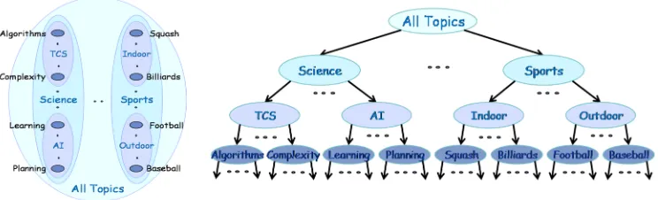
Figure 1: Consider a document clustering problem. Assume that data lies in multiple re-gions Algorithms, Complexity, Learning, Planning, Squash, Billiards, Football, Baseball. Suppose that the similarity K(x, y) = 0.999 if x and y belong to the same inner region; K(x, y) = 3/4 if x ∈ Algorithms and y ∈ Complexity, or if x ∈ Learning and y ∈ Planning, or if x ∈ Squash and y ∈ Billiards, or if x ∈ Football and y ∈ Baseball; K(x, y) = 1/2 if x is in (Algorithms or Complexity) andy is in (Learning or Planning), or ifxis in (Squash or Billiards) andy is in (Football or Baseball); define K(x, y) = 0 otherwise. Both clusterings

{Algorithms∪Complexity∪Learning∪Planning,Squash∪Billiards,Football∪

Baseball}and{Algorithms∪Complexity,Learning∪Planning,Squash∪Billiards∪

Football∪Baseball} satisfy the strict separation property.

2.1 Properties of the Similarity Function

We describe here some natural properties of the similarity functions that we analyze in this paper. We start with a noisy version of the simple strict separation property mentioned above (Balcan et al., 2008) and then define an interesting and natural generalization of it.

Property 1 The similarity function K satisfies ν-strict separation for the clustering problem (S, `) if for some S0 ⊆S of size (1−ν)n, K satisfies strict separation for (S0, `). That is, for all x, x0, x00∈S0 with x0 ∈C(x) and x00 6∈C(x) we have K(x, x0)>K(x, x00).

So, in other words we require that the strict separation is satisfied after a number of bad points have been removed. A somewhat different condition is to allow each point to have some bad immediate neighbors as long as most of its immediate neighbors are good. Formally:

Property 2 The similarity functionK satisfiesα-good neighborhood property for the clustering problem (S, `) if for all pointsx we have that all butαn out of theirnC(x) nearest

neighbors belong to the cluster C(x).

S; however, once we remove these points the remaining points are more similar to points in their own cluster than to points in other cluster. On the other hand, for the α-good neighborhood property we require that for all pointsxall butαnout of theirnC(x) nearest

neighbors belong to the cluster C(x). (So we cannot have a point that has similarity 1 to all the points in S.) Note however that different points might misbehave on different αn neighbors. We can also consider a property that generalizes both the ν-strict separation and theα-good neighborhood property. Specifically:

Property 3 The similarity function K satisfies (α, ν)-good neighborhood property for the clustering problem(S, `)if for some S0⊆Sof size (1−ν)n,K satisfiesα-good neighbor-hood for (S0, `). That is, for all points x∈S0 we have that all butαn out of their nC(x)∩S0 nearest neighbors in S0 belong to the cluster C(x).

Clearly, the (α, ν)-good neighborhood property is a generalization of both the ν-strict separation andα-good neighborhood property. Formally,

Fact 1 If the similarity function K satisfies the α-good neighborhood property for the clus-tering problem (S, `), then K also satisfies the (α,0)-good neighborhood property for the clustering problem (S, `).

Fact 2 If the similarity function K satisfies the ν-strict separation property for the clus-tering problem (S, `), then K also satisfies the (0, ν)-good neighborhood property for the clustering problem (S, `).

It has been shown that if K satisfies the ν-strict separation property with respect to the target clustering, then as long as the smallest target cluster has size 5νn, one can in polynomial time construct a hierarchy such that the ground-truth is ν-close to a pruning of the hierarchy (Balcan et al., 2008). Unfortunately the algorithm presented there is computationally very expensive: it first generates a large list of Ω(n2) candidate clusters and repeatedly runs pairwise tests in order to laminarize these clusters; its running time is a large unspecified polynomial. The new robust linkage algorithm we present in Section 3 can be used to get a simpler and much faster algorithm for clustering accurately under the ν-strict separation and the more general (α, ν)-good neighborhood property.

Generalizations Our algorithm succeeds under an even more general property called weak good neighborhood, which allows a good fraction of points to only have nice structure in their small local neighborhoods. The relations between these properties are described in Section 4.1, and the analysis under the weak good neighborhood is presented in Section 4.2.

2.2 Standard Linkage Based Algorithms Are Not Robust

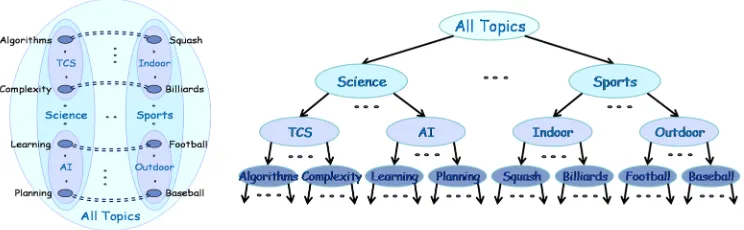
Figure 2: Same as Figure 1 except that let us match each point in Algorithms with a point in Squash, each point in Complexity with a point in Billiards, each point in Learning with a point in Football, and each point in Planning with a point in region Baseball. Define the similarities to be the same as in Figure 1 except that we letK(x, y) = 1 if x and y are matched. Note that for α= 1/n the similarity function satisfies the α-good neighborhood with respect to any of the prunings of the tree above. However, single linkage, average linkage, and complete linkage would initially link the matched pairs and produce clusters with very high error with respect to any such clustering.

in different inner blobs.2 See Figure 2 for a precise description of the similarity. In this example all the single linkage, average linkage, and complete linkage algorithms would in the first n/2 stages merge the matched pairs of points. From that moment on, no matter how they perform, none of the natural and desired clusterings will even be 1/2 close to any of the prunings of the hierarchy produced. Notice however, thatK satisfies theα-good neighborhood with respect to any of the desired clusterings (for α = 1/n), and that our algorithm will be successful on this instance. Theν-strict separation is not satisfied in this example either, for any constantν.

3. Robust Median Neighborhood Linkage

In this section, we propose a new algorithm, Robust Median Neighborhood Linkage, and show that it succeeds for instances satisfying the (α, ν)-good neighborhood property.

Informally, the algorithm maintains a threshold t and a list C0_t of subsets of points of S; these subsets are called blobs for convenience. We first initialize the threshold to a value t that is not too large and not too small (t= 6(α+ν)n+ 1), and initialize C_t0₋₁ to

Algorithm 1 Robust Median Neighborhood Linkage

Input: Similarity functionKon a set of pointsS,n=|S|, noise parametersα >0, ν >0.

Step 1 Initializet= 6(α+ν)n+ 1.

InitializeC_t0₋₁ to be a list of blobs so that each point is in its own blob. while|C0

t−1|>1 do

Step 2 B Build a graph Ft whose vertices are points in S and

whose edges are specified as follows.

Let Nt(x) denote the tnearest neighbors of x.

for any x, y∈S that satisfy |Nt(x)∩Nt(y)| ≥t−2(α+ν)ndo Connect x, yin Ft.

end for

Step 3 B Build a graph Ht whose vertices are blobs in Ct0−1 and

whose edges are specified as follows.

Let NF(x) denote the neighbors ofx inFt.

for any Cu, Cv ∈ Ct0−1 do

if Cu, Cv are singleton blobs, i.e., Cu ={x}, Cv ={y} then ConnectCu, Cv inHt, if|NF(x)∩NF(y)|>(α+ν)n.

else

SetSt(x, y) =|NF(x)∩NF(y)∩(Cu∪Cv)|, i.e., the number of points inCu∪Cv that are common neighbors ofx, y inFt. ConnectCu, Cv inHt, if medianx∈Cu,y∈CvSt(x, y)>

|Cu|+|Cv|

4 .

end if end for

Step 4 B Merge blobs in C_t0−1 to get Ct0 Set C_t0 =C_t0₋₁.

for any connected component V inHt with|S_C∈V C| ≥4(α+ν)ndo UpdateC0

t by merging all blobs inV into one blob.

end for

Step 5 B Increase threshold

t=t+ 1. end while

Output: Tree T with single points as leaves and internal nodes corresponding to the merges performed.

contain |S| blobs, one for each point in S. For each t, the algorithm builds C_t0 from C_t0₋₁

by merging two or more blobs as follows. It first builds a graph Ft, whose vertices are the data points inS and whose edges are constructed by connecting any two points that share at least t−2(α+ν)n points in common out of their t nearest neighbors. Then it builds a graph Ht whose vertices correspond to blobs in Ct0−1 and whose edges are specified in

pair of points x ∈ Cu, y ∈ Cv, it computes the number St(x, y) of points z ∈ Cu ∪Cv that are the common neighbors of x and y in Ft. It then connects Cu and Cv in Ht if medianx∈Cu,y∈CvSt(x, y) is larger than 1/4 fraction of |Cu|+|Cv|. Once Ht is built, we

analyze its connected components in order to create C0

t. For each connected component V of Ht, if V contains sufficiently many points from S in its blobs we merge all its blobs into one blob in C_t0. After building C_t0, the threshold is increased and the above steps are repeated until only one blob is left. The algorithm finally outputs the tree with single points as leaves and internal nodes corresponding to the merges performed. The full details of our algorithm are described in Algorithm 1. Our main result in this section is the following:

Theorem 1 Let K be a symmetric similarity function satisfying the (α, ν)-good neighbor-hood for the clustering problem(S, `). As long as the smallest target cluster has size greater than 6(ν +α)n, Algorithm 1 outputs a hierarchy such that a pruning of the hierarchy is

ν-close to the target clustering in time O(nω+1), where O(nω) is the state of the art for matrix multiplication.

In the rest of this section, we will first describe the intuition behind the algorithm in Section 3.1 and then prove Theorem 1 in Section 3.2.

3.1 Intuition of the Algorithm under the Good Neighborhood Property

We begin with some convenient terminology and a simple fact about the good neighborhood property. In the definition of the (α, ν)-good neighborhood property (see Property 3), we call the points in S0 good points and the points inB =S\S0 bad points. LetGi =Ci∩S0 be the good set of label i. Let G=∪_iGi denote the whole set of good points; so G=S0. Clearly |G| ≥n−νn. Recall that nCi is the number of points in the cluster Ci. Note that

the following is a useful consequence of the (α, ν)-good neighborhood property.

Fact 3 Suppose the similarity functionKsatisfies the(α, ν)-good neighborhood property for the clustering problem (S, `). As long as t is smaller than nCi, for any good point x∈Ci,

all but at most(α+ν)nout of its t nearest neighbors lie in its good set Gi.

Proof Letx∈Gi. By definition, out of its |Gi|nearest neighbors in G, there are at least

|Gi| −αn points fromGi. These points must be among its |Gi|+νn nearest neighbors in S, since there are at most νnbad points in S\G. This means that at most (α+ν)nout of its |Gi|+νn nearest neighbors are outside Gi. Notice |Gi|+νn≥nCi, we have that at

most (α+ν)n out of itsnCi nearest neighbors are outsideGi, as desired.

G1 G2 G3 G4

B

(a)F

G1

B

G2 G3 G4

(b) H

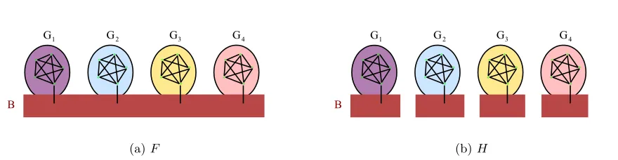
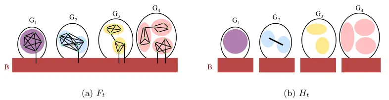
Figure 3: GraphF andH when all target clusters are of the same sizenC, which is known. InF, no two good points in different target clusters can be connected, and all good points in the same target cluster will be connected. InH, bad points connected to good points from different target clusters are disconnected.

simply output them. Alternatively, if there are bad points (ν >0), we can still cluster well as follows. We construct a new graph H on points in S by connecting points that share more than (α+ν)nneighbors in the graph F. The key point is that inF a bad point can be connected to good points from only one single target cluster. This then ensures that no good points from different target clusters are in the same connected component in H. So, if we output the largest kcomponents of H, we will obtain a clustering with error at most νn. See Figure 3 for an illustration.

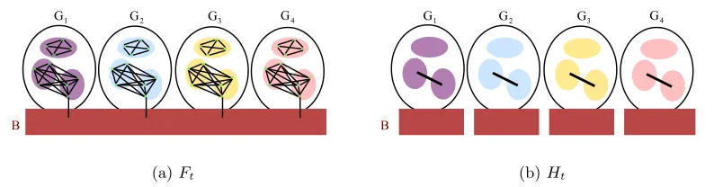
If we do not knownC, we can still use a pretty simple procedure. Specifically, we start with a thresholdt≤nC that is not too small and not too large (say 6(ν+α)n < t≤nC), and build a graph Ft on S by connecting two points if they share at least t−2(ν+α)n points in common out of theirtnearest neighbors. We then build another graphHtonS by connecting points if they share more than (α+ν)nneighbors in the graphFt. The key idea is that whent≤nC, good points from different target clusters share less thant−2(ν+α)n neighbors, and thus are not connected inFt andHt. If theklargest connected components of Ht all have sizes greater than (α+ν)n and they cover at least a (1−ν) fraction of the whole set of points S, then these components must correspond to the target clusters and we can output them. Otherwise, we increase the critical threshold and repeat. By the time we reachnC, all good points in the same target clusters will get connected inFtand Ht, so we can identify the klargest components as the target clusters.

G1 G2 G3 G4

B

(a)Ft

B

G1 G2 G3 G4

(b)Ht

Figure 4: GraphFt andHt when target clusters have the same sizenC but we do not know nC. The figure shows the case whent < nC. InFt, no good points are connected with good points outside their target clusters; inHt, blobs containing good points in different target clusters are disconnected.

blobs, it turns out that we can use a median test to outvote the noise.3 In particular, for two blobsCu andCv that are not both singleton, we compute for allx∈Cu andy∈Cv the quantitySt(x, y), which is the number of points inCu∪Cvthat are the common neighbors of xandyinFt. We then connect the two blobs inHtif medianx∈Cu,y∈CvSt(x, y) is sufficiently

large. See Figure 4 for an illustration and see Step 3 in Algorithm 1 for the details.

In the general case where the sizes of the target clusters are different, similar ideas can be applied. The key point is that when t ≤nCi, good points from Ci share less than

t−2(ν+α)nneighbors with good points outside, and thus are not connected to them inFt. Then inHt, we can make sure that no blobs containing good points inCi will be connected with blobs containing good points outside Ci. When t = nCi, good points in Ci form a

clique inFt, then all the blobs containing good points inCi are connected in Ht, and thus are merged. See Figure 5 for an illustration. Full details are presented in Algorithm 1 and the proof of Theorem 1 in the following subsection.

3.2 Correctness under the Good Neighborhood Property

In this subsection, we prove Theorem 1 for our algorithm. The correctness follows from Lemma 2 and the running time follows from Lemma 3. Before proving these lemmas, we begin with a useful fact which follows immediately from the design of the algorithm.

Fact 4 In Algorithm 1, for any t, if a blob in C_t contains at least one good point, then at least 3/4 fraction of the points in that blob are good points.

Proof This is clearly true when the blob is singleton. When it is non-singleton, it must be formed in Step 4 in Algorithm 1, so it contains at least 4(α+ν)npoints. Then the claim follows since there are at mostνnbad points.

G1 G2

G3

G4

B

(a)Ft

G1 G2

G3

G4

B

(b)Ht

Figure 5: Graph Ft and Ht when target clusters are of different sizes. The figure shows the case when t = nC2. In Ft, no good points are connected with good points

outside their target clusters; good points inC2 form a clique sincet=nC2. InHt,

blobs containing good points in different target clusters are disconnected; blobs containing good points inC2 are all connected.

Lemma 2 The following claims are true in Algorithm 1:

(1) For any Ci such that t ≤ |Ci|, any blob in Ct0 containing good points from Ci will not contain good points outside Ci.

(2) For any Ci such that t=|Ci|, all good points in Ci belong to one blob in Ct0.

Proof Before proving the claims, we first show that the graphFtconstructed in Step 2 has the following useful properties. Recall that Ft is constructed on points in S by connecting any two points that share at least t−2(α+ν)n points in common out of their t nearest neighbors. For anyCi such thatt≤ |Ci|, we have:

(a) If x is a good point in Ci and y is a good point outside Ci, then x and y are not connected inFt.

To see this, first note that by Fact 3, xhas at most (α+ν)nneighbors outsideCi out of the tnearest neighbors. For y ∈Gj, if nCj ≥t, theny has at most (α+ν)n

neighbors inCi; ifnCj < t,y has at most (α+ν)n+t−nCj neighbors inCi. In both

cases,y has at most (α+ν)n+ max(0, t−nCj)< t−5(α+ν)nneighbors inCi, since

nCj >6(α+ν)nandt >6(α+ν)n. Thenxandyhave at mostt−4(α+ν)ncommon

neighbors, so they are not connected inFt.

(b) If x is a good point inCi,y is a good point outsideCi, and z is a bad point, then z cannot be connected to both x andy inFt.

x _y

Cu Cv

B G

Figure 6: Illustration of the median test on Cu and Cv. At least 3/4 fraction of the points inCu and Cv are good points, and thus more than half of the pairs (x, y) with x∈Cu and y∈Cv are pairs of good points.

outsideCi. So they share less thant−2(α+ν)n+ 3(α+ν)n=t−2(α+ν)nneighbors and thus are not connected in Ft.

Now we prove Claim (1) in the lemma by induction on t. The claim is clearly true initially. Assume for induction that the claim is true for the threshold t−1 < |Ci|, that is, for any Ci such that t−1 <|Ci|, any blob in Ct0−1 containing good points from Ci will not contain good points outsideCi. We now prove that the graph Htconstructed in Step 3 has the following properties, which can be used to show that the claim is still true for the thresholdt.

• IfCu ∈ Ct0−1 contains good points fromCiandCv ∈ Ct0−1 contains good points outside

Ci, then they cannot be connected inHt.

If bothCuandCvare singleton blobs, sayCu ={x}, Cv ={y}, then by Property (a) ofFt, the common neighbors of x andy can only be bad points, and thus Cu and Cv cannot be connected.

If one of the two blobs (say Cu) is a singleton blob and the other is not, then Cu contains only one good point, and by Fact 4, at least 3/4 fraction of the points inCv are good points. If bothCu and Cv are non-singleton blobs, then by Fact 4, at least 3/4 fraction of the points inCu andCv are good points. Therefore, in both cases, the number of pairs (x, y) with good pointsx∈Cu andy ∈Cv is at least ₄3|Cu| ×3₄|Cv|>

|Cu||Cv|

2 . That is, more than half of the pairs (x, y) withx∈Cu and y ∈Cv are pairs

of good points; see Figure 6 for an illustration. This means there exist good points x∗ ∈Cu, y∗ ∈Cv such thatSt(x∗, y∗) is no less than medianx∈Cu,y∈CvSt(x, y). By the

induction assumption, x∗ is a good point in Ci and y∗ is a good point outside Ci. Then by Property (a)(b) of Ft,x∗ and y∗ have no common neighbors inFt, and thus medianx∈Cu,y∈CvSt(x, y) = 0. Therefore, Cu and Cv are not connected in Ht.

• If Cu ∈ Ct0−1 contains good points from Ci, Cv ∈ Ct0−1 contains good points outside

Ci, and Cw ∈ Ct0−1 contains only bad points, then Cw cannot be connected to both Cu and Cv in Ht.

in Step 4 in the algorithm and contain at least 4(α +ν)n points and thus cannot contain only bad points,Cw must be a singleton blob, containing only a bad pointz. Next, we show that if Cw = {z} is connected to Cu, then z must be connected to some good point in Ci in Ft. If Cu is a singleton blob, say Cu ={x}, then by Step 4 in the algorithm, z and x share more than (α+ν)n common neighbors in Ft. By Property (a)(b) ofFt, the common neighbors ofxandzinFtcan only be good points inCi or bad points. Since there are at most νn bad points, z must be connected to some good point in Ci in Ft. If Cu is not a singleton blob, then by Step 4 in the algorithm, medianx∈CuSt(x, z)>(|Cu|+|Cw|)/4. By Fact 4, at least 3/4 fraction of

the points in Cu are good points. So there exists a good point x∗ ∈ Cu such that St(x∗, z)≥medianx∈CuSt(x, z), which leads to St(x

∗_{, z)>(|C}

u|+|Cw|)/4> νn. By the induction assumption,x∗ is a good point inCi. Then by Property (a) of Ft,x∗ is only connected to good points from Ci and bad points. SinceSt(x∗, z) > νn, z and x∗ must share some common neighbors from Ci. Therefore, z is connected to some good point in Ci inFt.

Similarly, if Cw ={z} is connected to Cv, z must be connected to some good point outsideCi inFt. But thenzis connected to both a good point inCi and a good point outsideFt, which contradicts Property (b) of Ft.

By the properties ofHt, no connected component contains both good points inCi and good points outside Ci. So Claim (1) is still true for the threshold t. By induction, it is true for all thresholds.

Finally, we prove Claim (2). First, at the threshold t =|Ci|, all good points inCi are connected in Ft. This is because any good point in Ci has at most (α+ν)n neighbors outsideCi, so whent=|Ci|, any two good points inCi share at leastt−2(α+ν)ncommon neighbors and thus are connected inFt.

Second, all blobs in C0

t−1 containing good points in Ci are connected in Ht. There are two cases.

• If no good points in Ci have been merged, then all singleton blobs containing good points inCi will be connected in Ht.

This is because all good points in Ci are connected in Ft, and thus they share at least|Gi| ≥6(α+ν)n−νn points as common neighbors inFt.

• If some good points inCi have already been merged into non-singleton blobs inCt0−1,

we can show that inHtthese non-singleton blobs will be connected to each other and connected to singleton blobs containing good points from Ci.

Consider two non-singleton blobsCu andCv that contain good points fromCi. By Fact 4, at least 3/4 fraction of the points inCu andCv are good points. So there exist good points x∗ ∈Cu and y∗ ∈Cv such thatSt(x∗, y∗)≤medianx∈Cu,y∈CvSt(x, y). By

Claim (1),x∗ andy∗ must be good points inCi. Then they are connected to all good points inCi inFt, and thusSt(x∗, y∗) is no less than the number of good points inCu and Cv, which is at least 3(|Cu|+|Cv|)/4. Now we have medianx∈Cu,y∈CvSt(x, y) ≥

Therefore, in both cases, all blobs inC0

t−1 containing good points inCi are connected inHt. Then in Step 4, all good points inCi are merged into a blob in Ct0.

Lemma 3 Algorithm 1 has a running time of O(nω+1).

Proof The initializations in Step 1 take O(n) time. To compute Ft in Step 2, for any x ∈ S, let It(x, y) = 1 if y is within the t nearest neighbors of x, and let It(x, y) = 0 otherwise. Initializing It takes O(n2) time. Next we compute Nt(x, y), the number of common neighbors between x and y. Notice that Nt(x, y) =P_z∈SIt(x, z)It(y, z), so Nt= ItItT. Then we can compute the adjacency matrix Ft (overloading notation for the graph Ft) fromNt. These steps take O(nω) time.

To compute the graph Ht in Step 3, first define NSt=Ft(Ft)T. Then for two points x and y, NSt(x, y) is the number of their common neighbors in Ft. Further define a matrix F Ct as follows: if x and y are connected inFt and are in the same blob in Ct0−1, then let

F Ct(x, y) = 1; otherwise, let F Ct(x, y) = 0. As a reminder, for two points x that belongs toCu ∈ Ct0−1 and y that belongs to Cv ∈ Ct0−1, St(x, y) is the number of points in Cu∪Cv they share as neighbors in common inFt. F Ctis useful for computing St: since for x∈Cu and y∈Cv,

St(x, y) =

X

z∈Cv

Ft(x, z)Ft(y, z) +

X

z∈Cu

Ft(x, z)Ft(y, z)

= X

z∈S

Ft(x, z)F Ct(y, z) +

X

z∈S

F Ct(x, z)Ft(y, z),

we have St = Ft(F Ct)T +F Ct(Ft)T. Based on NSt and St, we can then build the graph Ht. All these steps takeO(nω) time.

When we perform merges in Step 4 or increase the threshold in Step 5, we need to recompute the above data structures, which takesO(nω) time. Since there areO(n) merges and O(n) thresholds, Algorithm 1 takes timeO(nω+1) in total.

4. A More General Property: Weak Good Neighborhood

In this section we introduce a weaker notion of good neighborhood property and prove that our algorithm also succeeds for data satisfying this weaker property.

To motivate the property, consider a pointxwith the following neighborhood structure. In the neighborhood of size n_C(x), x has a significant amount of its neighbors from other target clusters. However, in a smaller, more local neighborhood, x has most of its nearest neighbors from its target clustersC(x). In practice, points close to the boundaries between different target clusters typically have such neighborhood structure; for this reason, points with such neighborhood are called boundary points.

Planning

Learning Parameter Estimation

Hypothesis Testing

AI Statistics

(a)

Hypothesis Testing Parameter Estimation Planning Learning

Statistics AI

All Topics

(b)

AI Statistics

0.9

0.6 1.0

x y

0.9 0.9 0.6

(c)

Figure 7: Consider a document clustering problem. Assume that there are n/4 documents in each of the four areas: Learning, Planning, ParameterEstimation and Hypothe-sisTesting. The first two belong to the field AI, and the last two belong to the field Statistics. The similarities are specified as follows. (1) K(x, y) = 0.99 if x, y be-long to the same area; (2)K(x, y) = 0.8 ifx, ybelong to different areas in the same field; (3)K(x, y) = 0.5 ifx, ybelong to different fields. As shown in (b), there are four prunings: {Learning,Planning,ParameterEstimation,HypothesisTesting},

{AI,ParameterEstimation,HypothesisTesting}, {Learning,Planning,Statistics}, and {AI,Statistics}. All these four prunings satisfy the strict separation prop-erty, and consequently satisfy the α-good neighborhood property for α = 0. However, this is no longer true if we take into account noise that naturally arises in practice. As shown in (c), in each area, 1/8 fraction of the docu-ments lie close to the boundary between the two fields. More precisely, the similarities for these boundary documents are defined as follows. (1) These doc-uments are very similar to some document in the other field: for each bound-ary document x, we randomly pick one document y in the other field and set

K(x, y) =K(y, x) = 1.0; (2) These documents are also closely related to the other documents in the other field: K(x, y) = K(y, x) = 0.9 when x is a boundary document and y belongs to the other field; (3) These documents are not close to those in the other area in the same field: K(x, y) = K(y, x) = 0.6 when x is a boundary document and y belongs to the other area in the same field. Then the clustering{AI,Statistics}satisfies the (α, ν)-good neighbor property only for α ≥ 1/4 or ν ≥ 1/8. Similarly, {AI,ParameterEstimation,HypothesisTesting}

and {Learning,Planning,Statistics} satisfy the property only for α ≥ 1/4 or ν ≥ 1/16. See the text for more details, and see Section 6.1 for simulations of this example and its variants.

points, the clustering {AI,Statistics} satisfies the (α, ν)-good neighbor property only for α ≥ 1/4 or ν ≥ 1/8. This is because either we view all the boundary points as bad points in the (α, ν)-good neighborhood property which leads to ν ≥ 1/8, or we need α ≥ 1/4 since a boundary point has n/4 neighbors outside its target cluster. Similarly,

{AI,ParameterEstimation,HypothesisTesting} and {Learning,Planning,Statistics} satisfy the property only forα≥1/4 orν ≥1/16.

the desired clusterings ({Learning,Planning,ParameterEstimation,HypothesisTesting},

{AI,ParameterEstimation,HypothesisTesting},{Learning,Planning,Statistics}, and

{AI,Statistics}) are prunings of the hierarchy. As we show, the reason is that each of these prunings satisfies a generalization of the good neighborhood property which takes into account the boundary points, and for which our algorithm still succeeds. Note that the standard linkage algorithms fail on this example.4 In the following, we first formalize this property and discuss how it relates to the properties of the similarity function described in the paper so far. We then prove that our algorithm succeeds under this property, correctly clustering all points that are not adversarially bad.

For clarity, we first relax theα-good neighborhood to the weak (α, β)-good neighborhood defined as follows.

Property 4 A similarity functionK satisfies weak(α, β)-good neighborhood property for the clustering problem (S, `), if for each p ∈ S, there exists Ap ⊆ C(p) of size greater than 6αn such thatp∈Ap and

• any point inAp has at mostαnneighbors outsideAp out of the|Ap|nearest neighbors;

• for any such subset Ap ⊆C(p), at leastβ fraction of points in Ap have all but at most αn nearest neighbors from C(p) out of their nC(p) nearest neighbors.

Informally, the first condition implies that every point falls into a sufficiently large subset of its target cluster, and points in the subset are close to each other in the sense that most of their nearest neighbors are in the subset. This condition is about the local neighborhood structure of the points. It shows that each point has a local neighborhood in which points closely relate to each other. Note that the local neighborhood should be large enough so that the membership of the point is clearly established: it should have size comparable to the number of connections to points outside (αn). Here we choose a minimum size of greater than 6αn mainly because it guarantees that our algorithm can still succeed in the worst case. The second condition implies that for points in these large enough subsets, a majority of them have most of their nearest neighbors from their target cluster. This condition is about more global neighborhood structure. It shows how the subsets are closely related to those in the same target cluster in the neighborhood of size equal to the target cluster size. Note that in this more global neighborhood, we do not require all points in these subsets have most nearest neighbors from their target clusters; we allow the presence of (1−β) fraction of points that may have a significant number of nearest neighbors outside their target clusters.

Naturally, as we can relax the α-good neighborhood property to the (α, ν)-good neigh-borhood property, we can relax the weak (α, β)-good neighneigh-borhood to the weak (α, β, ν)-good neighborhood as follows. Informally, it implies that the target clustering satisfies the weak (α, β)-good neighborhood property after removing a few bad points.

4. For any fixed non-boundary point y and fixed boundary point x in the other field, the probability that yhas similarity 1.0 only withxis 2_n(1−2

n)

n/16−1_≈ 2

ne

−1/8

Property 5 A similarity function K satisfiesweak (α, β, ν)-good neighborhood prop-erty for the clustering problem (S, `), if there exist a subset of points B of size at most νn, and for eachp∈S\B, there exists Ap⊆C(p)\B of size greater than 6(α+ν)nsuch that p∈Ap and

• any point inAp has at mostαnneighbors outsideAp out of the|Ap|nearest neighbors;

• for any such subset Ap ⊆ Ci \B, at least β fraction of points in Ap have all but at mostαn nearest neighbors fromCi\B out of their|Ci\B|nearest neighbors inS\B.

For convenience, we call points in B bad points. If a point inCi\B has all but at most αn nearest neighbors from Ci\B out of its |Ci\B|nearest neighbors inS\B, we call it a good point. Then the second condition in the definition can be simply stated as: any Ap has at leastβ fraction of good points. Note thatCi can contain points that are neither bad nor good. Such points are called boundary points, since in practice such points typically lie close to the boundaries between target clusters.

As a concrete example, consider the clustering{AI,Statistics}in Figure 7(c). It satisfies the weak (α, β, ν)-good neighborhood property with probability at least 1−δ when the number of points n= O(ln1_δ). To see this, first note that for a fixed point y and a fixed boundary point x in the other field, the probability that K(y, x) = 1 is 2/n. Since there aren/16 boundary point in the other field, by Hoeffding bound, the probability thaty has similarity 1 with more thann/32 points is bounded by exp{−2·n/16·(1/2)2}= exp{−n/32}. By union bound, with probability at least 1−nexp{−n/32}, no point has similarity 1 with more thann/32 points. Then by setting Ap as the area thatpfalls in, we can see that the clustering satisfies the weak (α, β, ν)-good neighborhood property for α = 1/32, β = 7/8 and ν = 0. Note that there may also be some adversarial bad points. Then the weak (α, β, ν)-good neighborhood property is satisfied when α = 1/32, β = 7/8 and ν is the fraction of bad points. See Section 6.1 for simulations of this example and its variants.

4.1 Relating Different Versions of Good Neighborhood Properties

The relations between these properties are illustrated in Figure 8. The relations between the weak good neighborhood properties and other properties are discussed below, while the other relations in the figure follow from the facts in Section 2.1.

strict separation

−strict separation

−good neighborhood

, −good neighborhood

weak,−good neighborhood

weak,,−good neighborhood

By setting Ap = Ci for p ∈ Ci in the definition, we can see that the weak (α, β)-good neighborhood property is a generalization of theα-good neighborhood property when each target cluster has size greater than 6αn. Formally,

Fact 5 If the similarity function K satisfies the α-good neighborhood property for the clus-tering problem (S, `) and mini|Ci|>6αn, then K also satisfies the weak (α, β)-good neigh-borhood property for the clustering problem (S, `) for any0< β≤1.

Proof IfKsatisfies theα-good neighborhood property and mini|Ci|>6αn, then we have: for anyp∈Ci, there exists a subsetCi⊆Ci of size greater than 6αn, such that out of the nCi nearest neighbors, any pointx∈Ci has at mostαnneighbors outsideCi. SoKsatisfies

both conditions of the weak (α, β)-good neighborhood property.

By settingAp =Gi forp∈Gi in the definition, we can see that the weak (α, β, ν)-good neighborhood property generalizes the (α, ν)-good neighborhood property when each target cluster has size greater than 7(α+ν)n. Also, by setting ν = 0, we can see that the weak (α, β)-good neighborhood property is equivalent to the weak (α, β,0)-good neighborhood.

Fact 6 If the similarity function K satisfies the (α, ν)-good neighborhood property for the clustering problem(S, `) andmini|Ci|>7(α+ν)n, then K also satisfies the weak (α, β, ν) -good neighborhood property for the clustering problem (S, `) for any0< β≤1.

Proof If K satisfies the (α, ν)-good neighborhood property and mini|Ci| > 7(α+ν)n, then we have: for any p∈ Gi =Ci\B, there exists a subset Gi ⊆Gi of size greater than 6(α+ν)n, such that out of the |Gi|nearest neighbors inS\B, any good point x∈Gi has at mostαn neighbors outsideGi. SoK satisfies both conditions of the weak (α, β, ν)-good neighborhood property.

Fact 7 If the similarity function K satisfies the weak (α, β)-good neighborhood property for the clustering problem (S, `), then K also satisfies the weak (α, β,0)-good neighborhood property for the clustering problem (S, `).

Proof By settingν = 0 in the definition of the weak (α, β, ν)-good neighborhood property, we can see that it is the same as the weak (α, β)-good neighborhood property.

4.2 Correctness under the Weak Good Neighborhood Property

Now we prove that our algorithm also succeeds under the weak (α, β, ν)-good neighborhood property when β≥7/8. Formally,

A

4

A

A

1

A

A

3

A

6

Figure 9: Illustration of a fully formed blobCu: for any pointp∈Cu\B,Ap ⊆Cu. Then we can show that sets in{Ap:p∈Cu\B}are laminar, that is, for anyp, q∈Cu\B, eitherAp∩Aq =∅ or Ap ⊆Aq or Aq ⊆Ap. For example, in the figure we have Ap5 ⊆Ap4.

Theorem 4 is a generalization of Theorem 1, and the proof follows a similar reasoning. The proof of correctness is from Lemma 8 stated and proved below and the running time follows from Lemma 3. The intuition is as follows. First, by similar arguments as for the good neighborhood property, each point p in S\B will only be merged with other points inAp att≤ |Ap|, and all points in Ap will belong to one blob att=|Ap|(Lemma 5), since in the local neighborhood of size|Ap|, the point has most of its nearest neighbor from Ap. Then, we need to show that such blobs will be correctly merged. The key point is to show that even in the presence of boundary points, the majority of points in such blobs are good points (Lemma 7). Then the median test can successfully distinguish blobs containing good points from different target clusters, and our algorithm can correctly merge blobs from the same target clusters together.

To formally prove the correctness, we begin with Lemma 5. The proof is similar to that for Lemma 2, replacing Ci withAp.

Lemma 5 The following claims are true in Algorithm 1:

(1) For any pointp∈S\B and tsuch that t≤ |Ap|, any blob in C0t containing points from Ap will not contain points in (S\Ap)\B.

(2) For any point p∈S\B andt=|Ap|, all points inAp belong to one blob in Ct0.

Lemma 5 states that for anyp∈S\B, we will formApbefore merging them with points outside. Then we only need to make sure that these Ap formed will be correctly merged. More precisely, we need to consider the blobs that are “fully formed” in the following sense:

Definition 6 A blob Cu ∈ Ct0 in Algorithm 1 is said to be fully formed if for any point p∈Cu\B, Ap ⊆Cu.

Lemma 7 For any fully formed blob Cu ∈ Ct0 in Algorithm 1, at least β fraction of points in Cu\B are good points.

Proof It suffices to show that there exist a set of pointsP ⊆Cu\B, such that{Ap :p∈P} is a partition ofCu\B. ClearlyCu\B =∪p∈Cu\BAp. So we only need to show that sets in {Ap :p∈Cu\B} are laminar, that is, for anyp, q∈Cu\B, eitherAp∩Aq=∅orAp ⊆Aq orAq ⊆Ap. See Figure 9 for an illustration.

Assume for contradiction that there existAp andAq such thatAp\Aq 6=∅, Aq\Ap 6=∅ and Ap ∩Aq 6= ∅. Without loss of generality, suppose |Ap| ≤ |Aq|. Then by the second claim in Lemma 5, whent=|Ap|, all points inAp belong to one blob inCt0. In other words, this blob contains Ap∩Aq and Ap\Aq. So fort≤ |Aq|, the blob contains points inAq and also points inS\B\Aq, which contradicts the first claim in Lemma 5.

We are now ready to prove the following lemma that implies Theorem 4.

Lemma 8 The following claims are true in Algorithm 1:

(1) For anyCi such thatt≤ |Ci|, any blob inCt0 containing points inCi\B will not contain points in (S\Ci)\B.

(2) For any Ci such that t=|Ci|, all points in Ci\B belong to one blob in Ct0.

Proof Before proving the claims, we first show that the graphFtconstructed in Step 2 has the following useful properties by an argument similar to that in Lemma 2. Recall thatFt is constructed on points inS by connecting any two points that share at leastt−2(α+ν)n points in common out of their tnearest neighbors. For any Ci such thatt≤ |Ci|, we have:

(a) If x is a good point in Ci and y is a good point outside Ci, then x and y are not connected inFt.

To see this, first note that by Fact 3, xhas at most (α+ν)nneighbors outsideCi out of the t nearest neighbors. Suppose y is a good point from Cj. If nCj ≥t, then

y has at most (α+ν)nneighbors in Ci; ifnCj < t,y has at most (α+ν)n+t−nCj

neighbors inCi. In both cases,yhas at most (α+ν)n+max(0, t−nCj)< t−5(α+ν)n

neighbors inCi, sincenCj >6(α+ν)nandt >6(α+ν)n. Thenxand yhave at most

t−4(α+ν)n common neighbors, so they are not connected inFt.

(b) If x is a good point inCi,y is a good point outsideCi, and z is a bad point, then z cannot be connected to both x andy inFt.

Now we prove Claim (1) in the lemma by induction on t. The claim is clearly true initially. Assume for induction that the claim is true for the thresholdt−1, that is, for any Cisuch thatt−1≤ |Ci|, any blob inCt0−1 containing points inCi\B will not contain points in (S\Ci)\B. We now prove that the graph Ht constructed in Step 3 has the following properties, which can be used to show that the claim is still true for the thresholdt.

• IfCu ∈ Ct0−1contains points fromCi\BandCv ∈ Ct0−1contains points from (S\Ci)\B, then they cannot be connected inHt.

Suppose one of them (sayCu) is not fully formed, that is, there is a pointp∈Cu\B such thatAp 6⊆Cu. Then by Lemma 5, the algorithm will not mergeCuwithCvat this threshold. More precisely, since not all points inAp belong toCu, we havet−1<|Ap| by Claim (2) in Lemma 5. Then by Claim (1) in Lemma 5, sinceCv contains points in (S\Ap)\B,Cu andCv will not be merged inCt0. So they are not connected inHt. So we only need to consider the other case whenCu andCvare fully formed blobs. By Lemma 7, the majority of points in the two blobs are good points. The good points from different target clusters have few common neighbors in Ft, then by the median test in our algorithm, the two blobs will not be connected in Ht. Formally, we can find two good points x∗ ∈Cu, y∗ ∈Cv that satisfy the following two statements.

– St(x∗, y∗)≥medianx∈Cu,y∈CvSt(x, y).

By Lemma 7, at leastβ ≥7/8 fraction of points inCu\B are good points. The fraction of good points inCu is at least

β|Cu\B|

|Cu\B|+|B|

≥ 7/8×6(α+ν)n

6(α+ν)n+νn ≥ 3 4,

since|Cu\B| ≥6(α+ν)nand |B| ≤νn. Similarly, at least 3₄ fraction of points inCv are good points. Then among all the pairs (x, y) such thatx∈Cu, y∈Cv, at least 3₄ ×3

4 > 1

2 fraction are pairs of good points. So there exist good points

x∗ ∈Cu, y∗ ∈Cv such thatSt(x∗, y∗)≥medianx∈Cu,y∈CvSt(x, y).

– St(x∗, y∗)≤(|Cu|+|Cv|)/4.

The fraction of good points inCu∪Cv is at least 3₄. Since in Ft, good points in Cu are not connected to good points inCv, we haveSt(x∗, y∗)≤(|Cu|+|Cv|)/4.

Combining the two statements, we have medianx∈Cu,y∈CvSt(x, y) ≤ (|Cu|+|Cv|)/4

and thus Cu and Cv are not connected in Ht.

• If inC_t0₋₁,Cu contains points fromCi\B,Cv contains points from (S\Ci)\B, and Cw contains only bad points, then Cw cannot be connected to both Cu andCv.

By the same argument as above, we only need to consider the case when Cu and Cv are fully formed blobs. To prove the claim in this case, assume for contradiction that Cw is connected to both Cu and Cv. First, note the following fact about Cw. Since any non-singleton blob must be formed in Step 4 in the algorithm and contain at least 4(α+ν)n points and thus cannot contain only bad points, Cw must be a singleton blob, containing only a bad point z.

to at least one good point inCuinFt. We have medianx∈CuSt(x, z)>

|Cu|+|Cw|

4 , which

meanszis connected to more than |Cu|

4 points inCu inFt. By the same argument as

above, at least 3/4 fraction of points inCu are good points, thenzmust be connected to at least one good point inCu.

Similarly, if Cw is connected to Cv in Ht, then z must be connected to at least one good point in Cv in Ft. But this contradicts Property (b) of Ft, so Cw cannot be connected to bothCu and Cv in Ht.

By the properties of Ht, no connected component contains both points in Ci \B and points in (S\Ci)\B. So Claim (1) is still true for the thresholdt. By induction, it is true for all thresholds.

Finally, we prove Claim (2). By Lemma 5, when t = |Ci|, for any point p ∈ Ci \B, Ap belong to the same blob. So all points in Ci\B are in sufficiently large blobs. We will show that any two of these blobsCu, Cv are connected inHt, and thus will be merged into one blob. By Lemma 7, we know that more than 3/4 fraction of points in Cu (Cv respectively) are good points, and thus there exist good points x∗ ∈Cu, y∗ ∈Cv such that St(x∗, y∗)≤medianx∈Cu,y∈CvSt(x, y). By Claim (1), all good points inCu and Cv are from

Ci, so they share at least t−2(α+ν)n neighbors when t = |Ci|, and thus are connected in Ft. Then St(x∗, y∗) is at least the number of good points in Cu∪Cv, which is at least 3(|Cu|+|Cv|)/4. Then medianx∈Cu,y∈CvSt(x, y) ≥St(x

∗_{, y}∗_)>(|C

u|+|Cv|)/4. Therefore, all blobs containing points fromCi\B are connected inHtand thus merged into a blob.

5. The Inductive Setting

Many clustering applications have recently faced an explosion of data, such as in astrophysics and biology. For large data sets, it is often resource and time intensive to run an algorithm over the entire data set. It is thus increasingly important to develop algorithms that can remove the dependence on the actual size of the data and still perform reasonably well.

In this section we consider an inductive model that formalizes this problem. In this model, the given data is merely a small random subset of points from a much larger data set. The algorithm outputs a hierarchy over the sample, which also implicitly represents a hierarchy over the data set. In the following we describe the inductive version of our algorithm and prove that when the data satisfies the good neighborhood properties, the algorithm achieves small error on the entire data set, requiring only a small random sample whose size is independent of that of the entire data set.

5.1 Formal Definition

First we describe the formal definition of the inductive model. In this setting, the given data S is merely a small random subset of points from a much larger abstract instance space X. For simplicity, we assume that X is finite and that the underlying distribution is uniform over X. Let N =|X|denote the size of the entire instance space, and let n=|S|

Algorithm 2 Inductive Robust Median Neighborhood Linkage

Input: similarity function K,n∈Z+, parameters α >0, ν >0.

B Get a hierarchy on the sample

Sample i.i.d. examplesS ={x1, . . . , xn} uniformly at random fromX. Run Algorithm 1 with parameters (2α,2ν) on S and obtain a hierarchy T.

B Get the implicit hierarchy over X

for any x∈X do

LetNS(x) denote the 6(α+ν)n nearest neighbors of xinS. Initializeu= root(T) and fu(x) = 1.

whileu is not a leaf do

Letw be the child of uthat contains the most points in NS(x). Setu=w and fu(x) = 1.

end while end for

Output: Hierarchy T and {fu, u∈T}.

Our goal is to design an algorithm that based on the sample produces a hierarchy of small error with respect to the whole distribution. Formally, we assume that each nodeuin the hierarchy derived over the sample induces a cluster (a subset ofX). For convenience,u is also used to denote the blob of sampled points it represents. The cluster u induces over X is implicitly represented as a functionfu:X → {0,1}, that is, for eachx∈X,fu(x) = 1 ifx is a point in the cluster and 0 otherwise. We say that the hierarchy has error at most if it has a pruningfu1, . . . , fuk of error at most .

5.2 Inductive Robust Median Neighborhood Linkage

The inductive version of our algorithm is described in Algorithm 2. To analyze the al-gorithm, we first present the following lemmas showing that, when the data satisfies the good neighborhood property, a sample of sufficiently large size also satisfies the weak good neighborhood property.

Lemma 9 Let Kbe a symmetric similarity function satisfying the(α, ν)-good neighborhood for the clustering problem (X, `). Consider any fixedx∈X\B. If the sample size satisfies

n = Θ _α1 ln1_δ

, then with probability at least 1−δ, x has at most 2αn neighbors outside

(C(x)\B)∩S out of the |(C(x)\B)∩S| nearest neighbors in S\B.

Proof Supposex∈Gi. LetNN(x) denote its|Gi|nearest neighbors inX. By assumption we have that|NN(x)\Gi| ≤αN and |Gi\NN(x)| ≤αN. Then by Chernoff bounds, with probability at least 1−δ at most 2αnpoints in our sample are in NN(x)\Gi and at most 2αn points in our sample are inGi\NN(x).

points in (Gi \NN(x))∩S, and n3 be the number of points in (Gi∩NN(x))∩S. Then

|Gi∩S|=n2+n3 and we know that n1 ≤2αn,n2 ≤2αn. We consider the following two

cases.

• n1 ≥n2. Thenn1+n3 ≥n2+n3 =|Gi∩S|. This implies that the |Gi∩S|nearest neighbors ofx in the sample all lie inside NN(x), since by definition all points inside NN(x) are closer tox than any point outsideNN(x). But we are given that at most n1 ≤2αn of them can be outsideGi. Thus, we get that at most 2αn of the|Gi∩S| nearest neighbors of x are not fromGi.

• n1 < n2. This implies that the |Gi∩S| nearest neighbors ofx in the sample include allthe points inNN(x) in the sample, and possibly some others too. But this implies in particular that it includes all then3 points inGi∩NN(x) in the sample. So, it can include at most|Gi∩S| −n3=n2 ≤2αn points not inGi∩NN(x). Even if all those are not inGi, the|Gi∩S|nearest neighbors ofxstill include at most 2αnpoints not from Gi.

In both cases, at most 2αnof the|Gi∩S|nearest neighbors ofxinS\B can be outsideGi.

Lemma 10 Let K be a symmetric similarity function satisfying the (α, ν)-good neighbor-hood for the clustering problem(X, `). If the sample size satisfiesn= Θ_min(1_α,ν)ln_δmin(1_α,ν), then with probability at least 1−δ, K satisfies the (2α,2ν)-good neighborhood with respect to the clustering induced over the sample S.

Proof First, by Chernoff bounds, when n≥ 3

ν ln

2

δ, we have that with probability at least 1−δ/2, at most 2νnbad points fall into the sample.

Next, by Lemma 9 and union bound, whenn= Θ 1_αlnn_δwe have that with probability at least 1−δ/2, for anyCi, anyx∈Gi∩S,xhas at most 2αn points outsideGi∩S out of

its |Gi∩S|nearest neighbors in (X\B)∩S. Therefore, ifn= Θ

1 min(α,ν)ln

n δ

, then with probability at least 1−δ, the similarity function satisfies the (2α,2ν)-good neighborhood property with respect to the clustering induced over the sample S.

It now suffices to show n is large enough so thatn= Θ

1 min(α,ν)ln

n δ

. To see this, let η= min(α, ν). Since lnn≤tn−lnt−1 for any t, n >0, we have

c ηlnn≤

c η

η 2cn+ ln

2c η −1

= n 2 + c ηln 2c e·η,

for any constantc >0. Thenn= Θ

1 ηln 1 η

implies n= Θ

1

ηlnn

, andn= Θ

1

ηln

1

δ·η

implies n= Θ

1 η ln n δ .

Theorem 11 Let K be a symmetric similarity function satisfying the(α, ν)-good neighbor-hood for the clustering problem(X, `). As long as the smallest target cluster has size greater

than 12(ν+α)N, then Algorithm 2 with parameters n= Θ

1 min(α,ν)ln

1

δ·min(α,ν)

Proof Note that by Lemma 10, with probability at least 1−δ/4, we have thatK satisfies the (2α,2ν)-good neighborhood with respect to the clustering induced over the sample. Moreover, by Chernoff bounds, with probability at least 1−δ/4, each Gi has at least 6(ν+α)n points in the sample. Then by Theorem 1, Algorithm 1 outputs a hierarchy T on the sample S with a pruning that assigns all good points correctly. Denote this pruning as{u1, . . . , uk} such thatui\B = (Ci∩S)\B.

Now we want to show thatfu1, . . . , fuk have error at mostν+δ with probability at least

1−δ/2. For convenience, letu(x) be a shorthand ofu`(x). Then it is sufficient to show that

with probability at least 1−δ/2, a (1−δ) fraction of pointsx∈X\B have fu(x)(x) = 1.

Fix Ci and a point x∈Ci\B. By Lemma 9, with probability at least 1−δ2/2, out of the |Gi∩S| nearest neighbors of x in S\B, at most 2αn can be outsideGi. Recall that Algorithm 2 checksNS(x), the 6(α+ν)nnearest neighbors ofx inS. Then out of NS(x), at most 2(α+ν)npoints are outsideGi∩S. By Lemma 2,ui containsGi∩S, soui must contain at least 4(α+ν)n points inNS(x). Consequently, any ancestor w of ui, including ui, has more points in NS(x) than any other sibling of w. Then we must have fw(x) = 1 for any ancestor w of ui. In particular, fui(x) = 1. So, for any point x ∈ X\B, with

probability at least 1−δ2/2 over the draw of the random sample, fu(x)(x) = 1.

Then by Markov inequality, with probability at least 1−δ/2, a (1−δ) fraction of points x ∈X\B have f_u(x)(x) = 1. More precisely, let Ux denote the uniform distribution over X\B, and let US denote the distribution of the sample S. Let I(x, S) denote the event thatfu(x)(x)6= 1. Then we have

Ex∼Ux,S∼US[I(x, S)] =ES∼US

Ex∼Ux[I(x, S)|S]

≤δ2/2. Then by Markov inequality, we have

PrS∼US

Ex∼Ux[I(x, S)|S]≥δ

≤δ/2,

which means that with probability at least 1−δ/2 over the draw of the random sampleS, a (1−δ) fraction of pointsx∈X\B havefu(x)(x) = 1.

Similarly, Algorithm 2 also succeeds for the weak good neighborhood property. By similar arguments as those in Lemma 9 and 10, we can prove thatKsatisfies the weak good neighborhood property over a sufficiently large sample (Lemma 12), which then leads to the final guarantee Theorem 13. For clarity, the proofs are provided in Appendix B.

Lemma 12 Let K be a symmetric similarity function satisfying the weak (α, β, ν)-good neighborhood for the clustering problem (X, `). Furthermore, it satisfies that for any p ∈

X\B, |Ap|> 24(α+ν)N. If the sample size satisfies n= Θ

1 min(α,ν)ln

1

δmin(α,ν)

, then

with probability at least 1−δ, K satisfies the (2α,15₁₆β,2ν)-good neighborhood with respect to the clustering induced over the sample S.

Theorem 13 Let K be a symmetric similarity function satisfying the weak (α, β, ν)-good neighborhood for the clustering problem (X, `) with β ≥ 14

that for any p ∈ X \B, |Ap| > 24(α +ν)N. Then Algorithm 2 with parameters n =

Θ_min(1_α,ν)ln_δ·min(1_α,ν) produces a hierarchy with a pruning that is (ν +δ)-close to the target clustering with probability 1−δ.

6. Experiments

In this section, we compare our algorithm (called RMNL for convenience) with popu-lar hierarchical clustering algorithms, including standard linkage algorithms (Sneath and Sokal, 1973; King, 1967; Everitt et al., 2011), (Generalized) Wishart’s Method (Wishart, 1969; Chaudhuri and Dasgupta, 2010), Ward’s minimum variance method (Ward, 1963), CURE (Guha et al., 1998), and EigenCluster (Cheng et al., 2006).

To evaluate the performance of the algorithms, we use the model discussed in Section 2. Given a hierarchy output by an algorithm, we generate all possible prunings of sizek, where k is the number of clusters in the target clustering.5 Then we compute the Classification Error of each pruning with respect to the target clustering, and report the best error. The Classification Error of a computed clusteringhwith respect to the target clustering`is the probability that a point chosen at random from the data is labeled incorrectly.6 Formally,

err(h) = min σ∈Sk

Pr

x∈S[σ(h(x))6=`(x)]

,

where S_k is the set of all permutations on {1, . . . , k}. For reporting results, we follow the classic methodology (Guha et al., 1998): for all algorithms accepting input parameters (including (Generalized) Wisharts’ Method, CURE, and RMNL), the experiments are re-peated on the same data over a range of input parameter values, and the best results are considered.

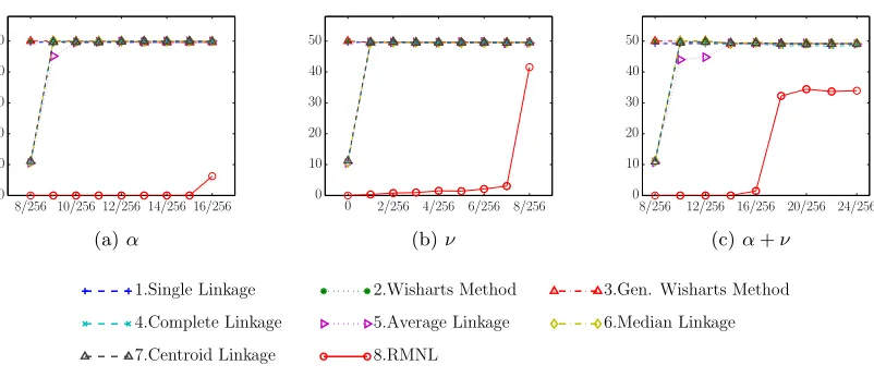
Data sets To emphasize the effect of noise on different algorithms, we perform controlled experiments on a synthetic data set AIStat. This data set contains 512 points. It is an instance of the example discussed in Section 4 and is described in Figure 7. We further consider the following real-world data sets from UCI Repository (Bache and Lichman, 2013): Wine, Iris, BCW (Breast Cancer Wisconsin), BCWD (Breast Cancer Wisconsin Diagnostic), Spambase, and Mushroom. We also consider the MNIST data set (LeCun et al., 1998) and use two subsets of the test set for our experiments: Digits0123 that contains the examples of the digits 0,1,2,3, and Digits4567 that contains the examples of the digits 4,5,6,7.

We additionally consider the 10 data sets (PFAM1 to PFAM10) (Voevodski et al., 2012), which are created by randomly choosing 8 families (of size between 1000 and 10000) from the biology database Pfam (Punta et al., 2012), version 24.0, October 2009. The sim-ilarities for the PFAM data sets are generated by biological sequence alignment software BLAST (Altschul et al., 1990). BLAST performs one versus all queries by aligning a queried sequence to sequences in the data set, and produces a score for each alignment. The score is a measure of the alignment quality and thus can be used as similarity. However, BLAST

5. Note that we generate all prunings of sizekfor evaluating the performance of various algorithms only. The hierarchical clustering algorithms do not need to generate these prunings when creating the hierarchies. 6. To compute this error for a computed clustering in polynomial time, we first find its best match to the target clustering using the Hungarian Method (Kuhn, 1955) for min-cost bipartite matching in time