Causal Bounds and Observable Constraints for Non-deterministic
Models
Roland R. Ramsahai [email protected]
Statistical Laboratory
Centre for Mathematical Sciences University of Cambridge
Wilberforce Road
Cambridge CB3 0WB, UK
Editor: Peter Spirtes
Abstract
Conditional independence relations involving latent variables do not necessarily imply observ-able independences. They may imply inequality constraints on observobserv-able parameters and causal bounds, which can be used for falsification and identification. The literature on computing such constraints often involve a deterministic underlying data generating process in a counterfactual framework. If an analyst is ignorant of the nature of the underlying mechanisms then they may wish to use a model which allows the underlying mechanisms to be probabilistic. A method of computation for a weaker model without any determinism is given here and demonstrated for the instrumental variable model, though applicable to other models. The approach is based on the analysis of mappings with convex polytopes in a decision theoretic framework and can be imple-mented in readily available polyhedral computation software. Well known constraints and bounds are replicated in a probabilistic model and novel ones are computed for instrumental variable mod-els without non-deterministic versions of the randomization, exclusion restriction and monotonicity assumptions respectively.
Keywords: instrumental variables, instrumental inequality, causal bounds, convex polytope, latent
variables, directed acyclic graph
1. Introduction
Conditional independence relations represent equality constraints on the parameters of a joint prob-ability distribution. Such relations cannot be empirically validated if they involve latent variables. Collections of latent conditional independencies may imply inequality constraints on parameters of the observable distribution. The classical motivation is the instrumental variable (IV) model (Durbin, 1954; Angrist et al., 1996). It includes the IV, A, and inference is required about the effect of a variable, B, on another, C, in the presence of latent confounders, U . The IV model is defined by A⊥⊥/ B, C⊥⊥A|(B,U)and U⊥⊥A. The latter two involve the latent variable U so it was tradition-ally thought that the model could not be empirictradition-ally verified (Imbens and Angrist, 1994). However Pearl (1995) derived the ‘instrumental inequality’
max
B
∑
C
max
A P(C,B|A)
a set of constraints which are implied by and can be used to falsify the discrete IV model. To compute the constraints, Pearl (1995) defines the IV model as a deterministic counterfactual model (Rubin, 1974). Such models involve latent deterministic relations, which marginalise to produce observed probabilistic relationships, and are technically equivalent to structural equation models (Strotz and Wold, 1960) and other functional models (Heckerman and Shachter, 1995).
Without intervention data and further assumptions, the causal effect of B on C cannot be point identified (Durbin, 1954; Angrist et al., 1996), but, using the deterministic counterfactual model, it can be bounded with the joint distribution of A, B and C (Pearl, 1995; Robins, 1989; Manski, 1990). Thus making it possible to acquire non-trivial information about the effect of the intervention when intervention studies cannot be conducted; because of ethical, financial or other reasons. Using the deterministic counterfactual approach and linear programming software developed by Balke (1995), the constraints on the causal effect of B on C were improved by Balke and Pearl (1997) and extended to other models by Kaufman et al. (2009). This linear programming approach within a deterministic counterfactual model has become the standard tool for computing such constraints, with some exceptions (Geiger and Meek, 1998; Kang and Tian, 2006).
As a technical construct for computations, deterministic counterfactual models are widely ac-cepted as valuable. Applications of deterministic counterfactual models assume there are underlying deterministic relations (Angrist et al., 1996) and pose no issues if the determinism can be practi-cally justified. For certain applications though, for example, mutations that cause cancer (Aalen and Frigessi, 2007), subject matter knowledge suggests that assumptions about the existence of deter-ministic mechanisms are unrealistic and spawns controversy (Dawid, 2000). Even if an analyst is unaware of the type of mechanisms involved in their study, it would be desirable to avoid determin-istic counterfactuals if alternative computations are no more difficult. The method in §2 provides such an alternative, which is agnostic to whether the underlying mechanisms are probabilistic or deterministic, to deriving falsifiable constraints and causal bounds of the type previously described. The method described does not use counterfactuals, which has certain advantages (Dawid, 2000), but more importantly demonstrates that the determinism in the models is unnecessary.
In this discussion, causal inference is formalized within standard decision theory (Spirtes et al., 1993; Pearl, 1993), with conditional independence assumptions (Lauritzen, 2001; Dawid, 2002). The model has been successfully applied in defining direct effects (Geneletti, 2007) and dynamic treatment strategies (Dawid and Didelez, 2010), to name a few. The approach in §2 and throughout uses this framework and it is compared to the counterfactual framework in §3. The method is based on the analysis of convex polytopes and can be implemented in standard polytope representation software such as Polymake (Gawrilow and Joswig, 2000) or PORTA (Christof and Loebel, 1998). Known constraints, which have been previously derived using deterministic counterfactuals, are derived in §5. Graphical models for representing causal assumptions are described in §4. Non-trivial modifications of the computation technique are considered in §6, §7 and §8 to derive novel constraints and causal bounds when various assumptions in the IV model are weakened.
The deterministic counterfactual framework only allows the compliance behaviour in Example 1 to be modelled as deterministic. Monotonicity assumptions, used to compute bounds in IV models, in the literature (Pearl, 1995; Balke and Pearl, 1997) are imposed in models which are stronger than necessary. It is shown in §8 that the known bounds and novel bounds can be derived for a weaker model. In the context of Example 1, monotonicity in the weaker model is equivalent to assuming that units are more likely to take treatment if assigned it than if not assigned it.
The counterfactual IV model in Example 1 uses the exclusion restriction assumption (Imbens and Angrist, 1994). This assumption restricts C to be a deterministic function of compliance be-haviour and treatment taken only. Stochastic exclusion restrictions are considered within the deter-ministic counterfactual framework in Hirano et al. (2000). In a weaker fully probabilistic model, the exclusion restriction assumption C⊥⊥A|(B,U)is used in §2 to replicate results which were derived under the stronger model (Balke and Pearl, 1993; Pearl, 1995; Balke and Pearl, 1997). Whilst vary-ing the strength of the exclusion restriction, novel constraints are derived in §7 with the probabilistic approach. This allows a sensitivity analysis to the non-deterministic exclusion restriction, which is important when assumptions involve unobservable variables (Shepherd et al., 2006).
Another assumption in the IV model in Example 1 is that treatment assignment is independent of compliance behaviour. In the probabilistic framework, novel constraints are computed for a weaker IV model with U⊥⊥/ A, as described in §6. Applications to data are given in §9. The IV model provides motivation for this discussion but the approach extends to other models. The notation used throughout is listed in Appendix A.
2. Computation of Constraints in the Instrumental Variable Model
Consider a model involving the random variables A, B, C and U , where the state space of A is {1,2}, B is {0,1} and C is {0,1}. U is unobservable by definition so no assumption is made about it. Let~v∗= (ζ∗00.1,ζ∗01.1, . . . ,ζ∗11.2) be a random vector with components ζ∗cb.a, which are random variables that are functions of U , whereζ∗cb.a=P(C=c,B=b|A=a,U). Similarly, let
~v= (ζ00.1,ζ01.1, . . . ,ζ11.2)be a fixed vector of probabilities that are not functions of U , whereζcb.a=
P(C=c,B=b|A=a). Let~τ∗= (η∗
0,η∗1,δ∗1,δ∗2), where η∗
b=P(C=1|B=b,U), δa∗=P(B=1|A=a,U). (2)
Since~τ∗is a vector of probabilities then~τ∗∈
T
since the components of~τ∗satisfy the axioms of probability, whereT
= [0,1]4. To derive falsifiable constraints on~v for the IV model, it is necessary to determine the set of~v which does not satisfy the assumptions in the IV model. Under the IV model, C⊥⊥A|(B,U), which implies thatP(C,B|A,U) =P(C|B,U)P(B|A,U), (3)
and~v∗can be parameterised by~τ∗. The relation in Equation (3) together with the codes in (2) define a mappingΞ:~τ∗∈
T
→~v∗∈V
, where~τ∗is unrestricted by the IV model andV
=Ξ(T
)contains all~v∗which obey the IV model. Since the components of each~v∗ obey the axioms of probability thenV
⊆Z
, whereZ
⊂[0,1]8is the intersection of the hyperplanes defined by ∑c,bζ∗cb.a=1 for
a∈ {1,2}.
Under the IV model, U⊥⊥A, which implies thatζcb.a=EU(ζ∗cb.a)and thus all~v that obey the IV
hull of
V
. Let ˆV
=Ξ(T
ˆ)and ˆH
be the convex hull of ˆV
, where ˆT
is the collection of extreme vertices ofT
. The vertices ˆT
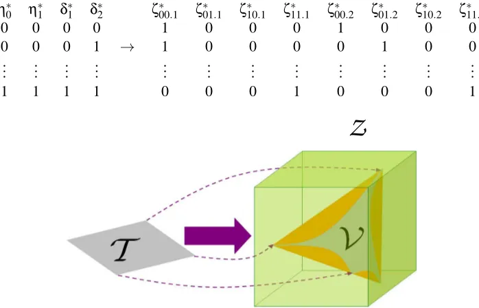
and ˆV
are partially listed in Figure 1 (top) and the transformation Ξ(·)is represented in Figure 1 (bottom).η∗
0 η∗1 δ∗1 δ∗2 ζ00∗ .1 ζ∗01.1 ζ∗10.1 ζ∗11.1 ζ∗00.2 ζ∗01.2 ζ∗10.2 ζ∗11.2
0 0 0 0 1 0 0 0 1 0 0 0
0 0 0 1 → 1 0 0 0 0 1 0 0
..
. ... ... ... ... ... ... ... ... ... ... ...
1 1 1 1 0 0 0 1 0 0 0 1
Z
Figure 1: Transformation of extreme vertices (top) of polytope (bottom).
Since
H
=H
ˆ , from Theorem 1 in Appendix B, then all~v that obey the IV model lie in ˆH
. The proof of Theorem 1 does not use the specific form ofΞ(·), only its monotonicity in each coordinate. A program such as Polymake (Gawrilow and Joswig, 2000) or PORTA (Christof and Loebel, 1998) can be used to transform the representation of ˆH
in terms of its extreme vertices to a representation in terms of its facets or inequalities. The inequalities are constraints which are satisfied by~v if~v obeys the IV model. This specific computation produces the falsifiable ‘instrumental inequality’ constraints in (1) and is exactly the approach of Dawid (2003).It is possible for the randomization or exclusion restriction assumption to fail without violation of any of the constraints in (1). This is because there are distributions P(C,B,A,U)which either violate the assumption U⊥⊥A or Equation (3) but give rise to margins P(C,B,A) that obey the inequalities in (1). For example, if all~v∗lie in
H
\V
and randomization holds then the exclusion restriction in Equation (3) is not satisfied but all~v∈H
, which means that the inequalities in (1) are satisfied. I conjecture that the condition that U has a certain small state space is sufficient to imply that it is possible for the IV model to fail without violation of any of the constraints in (1).3. Geometry of Counterfactuals and Latent Variables
The binary IV model can be re-parameterised by replacing U in P(C,B|A,U)with~τ∗ and consid-ering P(C,B|A,~τ∗). The polytope
H
represents the model for P(C,B|A) and, sinceH
=H
ˆ , a computationally and empirically indistinguishable model is formed by restricting~τ∗ to ˆT
. In this minimal representation of the model, where~τ∗∈T
ˆ, the parametersη∗b∈ {0,1}andδ∗a ∈ {0,1}.
a counterfactual variable which is the value of C when B=b for a given~τ∗, and similarly forδ∗
a.
Similar comments are given in Lauritzen (2004).
If U is interpreted as the collection of variables which define a unit then~τ∗ is the vector of potential responses for a unit and each vertex of the polytope corresponds to a certain type of unit. In the partial compliance model of Example 1, the vertex~τ∗= (0,0,0,0) corresponds to a unit which is classified as never recover (response is 0 regardless of treatment taken) and a never taker (treatment taken is 0 regardless of treatment assigned).
The probabilistic model is parameterised by~τ∗over the entire polytope
T
whereas the counter-factual model is parameterised by~τ∗only at the extreme vertices of the polytopeT
. In special cases where latent determinism is realistic then such a parameterisation is meaningful and assumptions about the non-existence of certain vertices of the polytope or~τ∗∈T
ˆ can potentially be justified. If latent determinism is known to be unrealistic (Aalen and Frigessi, 2007) and the reparameterisation is a technical construct then it may be wise to steer clear of any interpretation beyond simply saying that they are the vertices of the polytope defining the model.The concepts are demonstrated in the reformulation of the monotonicity assumption in §8. The deterministic counterfactual approach assumes latent determinism and interprets the vertices as hav-ing real meanhav-ing. Under the deterministic interpretation, the monotonicity assumption implies that certain vertices are not valid for the model. The probabilistic approach defines monotonicity as a constraint on the latent conditional distributions to lie in a particular half-space, still allowing probabilistic behaviour.
4. Causal Graphical Models
The IV model considered so far, that is, without causal assumptions, is relatively simple. However extensions of it will be considered later and it will be useful, though not vital, to use graphical models to represent the assumptions involved. Graphs that are useful for representing conditional independence and causal assumptions are described in §4.1 and §4.2 respectively.
4.1 Directed Acyclic Graph
A purely probabilistic directed acyclic graph (DAG) (Lauritzen, 1996) consists of a set of vertices or nodes,
N
, and a set of directed edges,E
. Ifλ1,λ2∈N
and(λ1,λ2)∈E
then(λ2,λ1)∈/E
. It is said that there is a directed edge fromλ1toλ2, this is written asλ1→λ2andλ1is called a parent ofλ2. In a DAG which represents the probability distribution of a set of random variables,X
, every λ∈N
corresponds to a random variableX
λ∈X
. The probability distribution function has the formP(
X
) =∏λ∈N P{X
λ|X
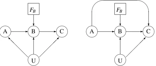
pa(λ)}, (4) where ‘pa(·)’ is the set of ‘parents’ of a node. This factorisation property is equivalent to a collection of conditional independence relations, which can be derived from the DAG using the concepts of ‘d-separation’ (Verma and Pearl, 1988) and a ‘moral graph’ (Lauritzen et al., 1990). The observational assumptions of the IV model can be represented by the DAG in Figure 2 (left).4.2 Augmented Directed Acyclic Graph
A
B
C
U
6
A
B
C
6
U
FB
Figure 2: DAG which represents observational assumptions of the instrumental variable model (left) and augmented DAG for IV model, which includes causal assumptions (right).
the notation, P(C||B=b)is the probability of C given that B is actively forced to take the value b, and not passively observed to take the value b, as in P(C|B=b).
To derive intervention constraints, the assumptions represented by the augmented DAG (Spirtes et al., 1993; Pearl, 1993; Lauritzen, 2001; Dawid, 2002) in Figure 2 (right) are considered, where ACE(B→C) =α=P(C=1||B=1)−P(C=1||B=0) is the causal effect of interest. The intervention node FB is a regime indicator decision variable which represents the way in which
the value of B arises. Conditional independence relations can be derived in the same way as for the purely probabilistic DAGs since the probability distribution, conditional on FB, still factorises
according to Equation (4). The node FBtakes the values ‘idle’, 0 or 1. If FB=idle then B takes a
random value given by P{B|pa(B)}, but if FBis either 0 or 1 then B=FB. Using previous notation
P(C||B=b) =P(C|FB=b). The relation C⊥⊥B|(FB=b,U)holds from the definition of FBbut is
not represented in Figure 2 (right). Square nodes are decision nodes which represent fixed strategies, whereas circle nodes are random nodes which represent random variables.
The augmented DAGs which represent the IV model without randomization and the exclusion restriction are given in Figure 3.
A
B
C
@ @ @ @
I 6
U
?
FB
A
B
C
' $
?
6
U
?
FB
Figure 3: Augmented DAGs which represent the causal IV model without randomization (left) and without exclusion restriction (right).
5. Applications of Computation
Many results in the literature are recovered by specific applications of the general method described in §2. It is based on parameterising with the factors of Equation (4) and transforming them according to a mapping. By defining the appropriate mapping, the various constraints are obtainable. Key requirements are the monotonicity of the mapping and that the space of valid parameters is the convex hull of the transformed polytope. Constraints on other quantities, such as P(C|A), P(B|A), P(C|B)etc., can be derived but some interesting examples are given in §5.1 and §5.2.
5.1 Falsifiable Constraints
Some applications, such as studies with partial compliance, require constraints involving the distri-bution P(C,B|A), whereas others can only identify the pairwise conditional distributions P(C|A) and P(B|A). For example, Mendelian randomization in genetic epidemiology involves the use of a genotype (A) as an instrument for the effect of a phenotype (B) on a disease (C). However only genotype-phenotype and genotype-disease data is usually available (Didelez and Sheehan, 2007) and thus constraints involving P(C|A)and P(B|A)are needed.
To derive the constraints, consider the monotone mapping~τ∗ 7−→(~γ∗,~θ∗)for the IV model of Figure 2 (left), whereγ∗ca=P(C=c|A=a,U) andθ∗ba=P(B=b|A=a,U). Since U⊥⊥A then (~γ,~θ)lies in the convex hull of the set of(~γ∗,~θ∗)which satisfy the IV model, whereγ
ca=P(C=
c|A=a)andθba=P(B=b|A=a). Similarly to the approach in §2, the constraints
θ01+θ02≥γ01−γ02, θ01+θ02≥γ02−γ01, θ11+θ12≥γ01−γ02, θ11+θ12≥γ02−γ01, are obtained, which are the same as in Ramsahai (2007).
5.2 Bounds on Fixed Interventions
From the motivating Mendelian randomization example in §5.1, it may be necessary to obtain causal bounds in terms of the pairwise conditional distributions P(C|A)and P(B|A). Consider the model in Figure 2 (right). Since C⊥⊥FB|(B,U) and U⊥⊥FB then P(C||B) =∑UP(C|B,U)P(U). This
implies that(~γ,~θ,α)lies in the convex hull of(~γ∗,~θ∗,α∗), whereα∗=P(C=1|B=1,U)−P(C= 1|B=0,U)andα=EU(α∗). Therefore the monotone mapping~τ∗7−→(~γ∗,~θ∗,α∗)can be used to
compute constraints on(~γ,~θ,α). The results of the computation are given in Appendix C and are the same as those derived in Ramsahai (2007).
Similarly, constraints and causal bounds in terms of the identifiable ζcb.a parameters can be
obtained by considering the mapping~τ∗ 7−→ (~v∗,α∗). The constraints involving the identifiable
ζcb.a parameters only are the same as those obtained in §2, which are given in (1), and the rest
constrainα. The bounds onαare given in Appendix C and are the same as those of Dawid (2003), which are derived by Balke and Pearl (1997) in a deterministic model.
6. Relaxing the Randomization Assumption in the Instrumental Variable Model
status of the patients. To analyze such a study, an analyst may opt for a model without randomization or at least assess the effect of the assumption on the inference. Both require constraints to be derived for a model without U⊥⊥A, as in Figure 3 (left). The decision framework is used here for computations without any assumptions of determinism. It is irrelevant to the computation whether U causes A, A causes U or both have a common cause. This is because the model in Figure 3 (left) only makes assumptions about distributions in the observational regime and the regime with intervention on B, since it includes the regime indicator FB. No FA or FU regime indicators are
included so no assumptions are made about interventions on A or U .
If there is data on P(C|A)and P(B|A)but not P(C|B,A)then constraints and bounds involving
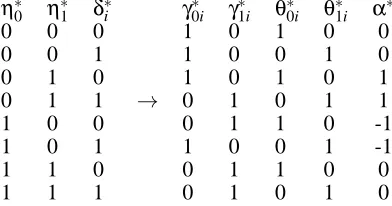
~γand~θare useful. Without the randomization assumption, U⊥⊥A, (~γ,~θ,α) does not necessarily lie in the convex hull of (~γ∗,~θ∗,α∗) and similarly for the other applications in §5. Assuming the exclusion restriction in Equation (3) still holds,~τ∗still fully parameterises P(C,B|A,U). Consider the monotone mappingΞi(·):~τ∗7−→~vi∗, where~vi∗= (γ∗0i,γ∗1i,θ∗0i,θ1i∗,α∗)for i=1,2, which can be expressed as
α∗=η∗
1−η∗0, γ∗0i= (1−η∗0)(1−δ∗i) + (1−η∗1)δ∗i, θ∗0i=1−δ∗i
γ∗
1i=η∗0(1−δ∗i) +η1∗δ∗i, θ∗1i=δ∗i.
The transformation of ˆ
T
byΞi(·)is given in Figure 4. Since the relations C⊥⊥FB|(B,U), U⊥⊥FBη∗
0 η∗1 δ∗i γ∗0i γ∗1i θ∗0i θ∗1i α∗
0 0 0 1 0 1 0 0
0 0 1 1 0 0 1 0
0 1 0 1 0 1 0 1
0 1 1 → 0 1 0 1 1
1 0 0 0 1 1 0 -1
1 0 1 1 0 0 1 -1
1 1 0 0 1 1 0 0
1 1 1 0 1 0 1 0
Figure 4: Transformation of ˆ
T
by Ξi(·) to the polytope which represents the IV model withoutrandomization, in terms of the pairwise conditional distributions P(C|A)and P(B|A).
and C⊥⊥A|(B,U)follow from Figure 3 and C⊥⊥B|(U,FB=B),
P(C||B) =∑A∑UP(C|B,U)P(U|A)P(A) =EA(α′A), (5)
whereα′A=∑UP(C|B,U)P(U|A). Since P(C|A) =EU|A{P(C|A,U)}and P(B|A) =EU|A{P(B|A,U)}
then~wilies in the convex hull of the set of~vi∗, where~wi= (γ0i,γ1i,θ0i,θ1i,α′i), and the method of §2
computes the tight constraints
0≤γ0i+2γ1i−θ0i+α′i,
0≤γ0i+θ0i+α′i,
0≤γ1i+θ0i−α′i,
0≤2γ0i+γ1i−θ0i−α′i,
or
for all i. The constraints are tight since the vertices of the convex hull are a subset of the vertices of the transformed polytope and any vertex is achievable if the value of U , corresponding to the vertex, occurs with probability one. Sinceα=EA(α′A)from Equation (5) then
min
i
max
γ0i+θ0i−2 −γ0i−θ0i
≤α≤max
i
min
−γ0i+θ0i+1 γ0i−θ0i+1
.
These bounds always span zero and are tight since the bounds onα′iare achievable byαif P(A= i) =1. If marginal A data are available, the bounds can be improved to
ACE(B→C)≥∑i
max
γ
0i+θ0i−2 −γ0i−θ0i
P(A=i)
,
ACE(B→C)≤∑i
min
−γ0i+θ0i+1 γ0i−θ0i+1
P(A=i)
,
or
−1+EA(|γ1A−θ0A|)≤ACE(B→C)≤1−EA(|γ0A−θ0A|). (6) Although the expression in (6) bounds the unobservable causal effect, there are no falsifiable con-straints to invalidate the model. The bounds in (6) always span zero.
If a sample from P(C,B|A)is available, the mapping~τ∗7−→~v∗
i can be used to compute
observ-able constraints and causal bounds. The computation is possible since P(C,B|A) = EU|A{P(C,B|A,U)}, which implies that~wi lies in the convex hull of the set of~vi∗, where~vi∗=
(ζ∗
00.i,ζ∗01.i,ζ∗10.i,ζ∗11.i,α∗)and~wi= (ζ00.i,ζ01.i,ζ10.i,ζ11.i,α′i). The bounds−ζ01−ζ10≤ACE(B→ C)≤ζ00+ζ11are obtained, whereζcb=P(C=c,B=b). All of the results in this section still hold
if the state space of A is extended to{1,2, . . . ,l}but the state space of(B,C)kept binary.
The bounds on ACE(B→C)by the ζcb parameters are derived by Manski (1990) in a model
involving (B,C,C0,C1) under the assumptions that the potential outcomes (C0,C1) for a unit are the same regardless of how treatment is assigned, that is, whether by intervention or observation, and thus C is a deterministic function of(B,C0,C1) for a unit. The derivation, of the bounds on ACE(B→C) by theζcb parameters, given here only requires the analogous assumptions U⊥⊥FB
and C⊥⊥FB|(B,U). The additional variable A used here, which satisfies the condition C⊥⊥A|(B,U),
trivially exists by constructing a variable A=B. Also, the conditional independence assumption A⊥⊥FBrepresented in Figure 3 (left) is unnecessary since it is not used in the derivation.
7. Relaxing the Exclusion Restriction in the Instrumental Variable Model
The exclusion restriction assumption may often be inapplicable, for example, if patients in a study with partial compliance become aware of their treatment assignment and this affects their outcome. There could be a direct relation between treatment assignment A and the outcome C, for which the model in Figure 3 (right) would be appropriate. The probabilistic nature of the exclusion restric-tion within the decision framework allows the strength of the direct relarestric-tion to be varied and the sensitivity of inference to this assumption to be assessed.
η∗
01 η∗02 η∗11 η∗12 δ∗1 δ∗2
0 0 0 0 0 0
0 0 0 0.5 0 1 0 0 0.5 0 1 0 0 0 0.5 1 1 1 0 0 1 0.5 0 0
0 0 1 1 0 1
..
. ... ... ... ... ...
↓
ζ∗
00.1 ζ∗01.1 ζ∗10.1 ζ∗11.1 ζ∗00.2 ζ∗01.2 ζ∗10.2 ζ∗11.2
1 0 0 0 1 0 0 0
1 0 0 0 0 0.5 0 0.5 0 0.5 0 0.5 1 0 0 0 0 0.5 0 0.5 0 0 0 1
1 0 0 0 1 0 0 0
1 0 0 0 0 0 0 1
..
. ... ... ... ... ... ... ...
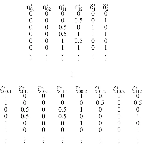
Figure 5: Transformation to the extreme vertices corresponding to the polytope which represents the IV model with the weaker exclusion restriction, forε=0.5, in terms of the distribution P(C,B|A).
The conditionε=0 is equivalent to the exclusion restriction. Forε=1, there are no constraints on(η∗b1,η∗b2)other than the axioms of probability and there are no falsifiable constraints or causal bounds for the IV model without the exclusion restriction. The augmented DAG in Figure 3 (right) does not represent any assumptions aboutεbut assumptions aboutεare required to obtain non-trivial constraints and bounds. The application of the technique is considered forε=0.5. Consider the mapping of~τ∗= (η∗
01,η∗02,η∗11,η12∗ ,δ∗1,δ∗2)to~v∗= (ζ∗00.1,ζ∗01.1, . . . ,ζ∗11.2)for a model with A∈ {1,2} and B,C∈ {0,1}. The transformation of some of the extreme vertices are given in Figure 5. Use of the technique produces the causal bounds in Appendix D and the constraints
ζ00.1+ζ10.2−ζ10.1−ζ00.2≤1, ζ10.1+ζ00.2−ζ00.1−ζ10.2≤1, ζ11.1+ζ01.2−ζ01.1−ζ11.2≤1, ζ01.1+ζ11.2−ζ11.1−ζ01.2≤1,
which is a weaker version of the ‘instrumental inequality’ of Equation (1) and can be violated if the IV model with the weak exclusion restriction, ε=0.5, is invalid. By adding the component P(C|B,A,U) to~v∗, causal bounds on P(C|A,FB=B) =∑UP(C|B,A,U)P(U)can be derived for
each A and used to compute bounds on ACE(B→C)since P(C|FB=B) =∑AP(C|A,FB=B)P(A).
7.1 Bounds on Direct Effects
Without assuming C⊥⊥A|(B,U), if intervention on A is possible then the direct effect of A on C can be bounded with parameters of the distribution under no intervention. Consider extending the sample space of FB to include the random regime dA, which represents the regime in which
P(B|A,U,FB=da∗) =P(B|A=a∗,U). Consider the controlled direct effect (CDE) (Didelez et al.,
2006) and the random regime direct effect (RRDE)
CDE(B) = E(C|FB=B,FA=2)−E(C|FB=B,FA=1)
= EU{E(C|B,A=2,U)−E(C|B,A=1,U)}
= EU(η∗B2−η∗B1),
RRDE(a∗) = E(C|FB=da∗,FA=2)−E(C|FB=da∗,FA=1)
= EU[EB{E(C|B,A=2,U)−E(C|B,A=1,U)|A=a∗,U}]
= EU{(η∗12−η∗11)δ∗a∗+ (η∗12−η∗11)(1−δ∗a∗)}.
The RRDE is called the NDE in Didelez et al. (2006) but Robins and Richardson (2010) argue that the parameter being referred to as NDE in Didelez et al. (2006) is not the same as the NDE in Pearl (2001). Thus a separate name is given here to RRDE. By considering the mapping of~τ∗ to the vector with~v∗and the extra componentη∗B2−η∗
B1, the bounds on CDE(B)of Cai et al. (2008) can
be replicated. Similarly by mapping~τ∗to a vector with~v∗and E
B(η∗B2−ηB1∗ |A=a∗,U), bounds on
RRDE(a∗)are obtained, which are identical to the bounds on NDE(a∗)in Sj¨olander (2009). Unlike here, both references use counterfactuals and use the definition of CDE and NDE, sometimes called pure direct effect (Robins and Greenland, 1992), given in Pearl (2001).
8. Monotonicity Assumption in the Instrumental Variable Model
The monotonicity assumption in the literature (Imbens and Angrist, 1994; Angrist et al., 1996) is formulated in a deterministic model. In a partial compliance study, a patient may be more likely to take treatment under assignment but it may not be reasonable to assume that their behaviour is deterministically related to treatment assignment. A monotonicity assumption in a weaker proba-bilistic model is considered here and can be expressed mathematically for the binary IV model by δ∗
2≥δ∗1, from Equation (2). It restricts the space of the vector of probabilities so the constraints are at least as strong as without it.
The IV model considered in this section includes the exclusion restriction and the randomization assumption, as in the augmented DAG in Figure 2 (right). As an illustrative example, consider the computation of falsifiable constraints and causal bounds onϕgiven~γ, without monotonicity, where ϕ=ACE(A→B) =θ01−θ02. This computation produces only trivial results. Under monotonicity,
T
must be redefined to omit all~τ∗which do not satisfy it. Therefore all of the vertices withδ∗ 2<δ∗1 orϕ∗≥0 should be removed to redefine ˆT
, whereϕ∗=P(B=1|A=2,U)−P(B=1|A=1,U). The required mapping is~τ∗7−→(~γ∗,ϕ∗)over the domain of the restrictedT
. The transformation is given in Figure 6 and the non-trivial constraints obtained aremax
γ
01−γ02 −γ01+γ02
η∗
0 η∗1 δ∗1 δ∗2 γ01∗ γ∗11 γ∗02 γ∗12 ϕ∗
0 0 0 0 1 0 1 0 0
0 0 0 1 1 0 1 0 1
0 0 1 0 − − − − −
0 0 1 1 1 0 1 0 0
0 1 0 0 1 0 1 0 0
0 1 0 1 1 0 0 1 1
0 1 1 0 − − − − −
0 1 1 1 → 0 1 0 1 0
1 0 0 0 0 1 0 1 0
1 0 0 1 0 1 1 0 1
1 0 1 0 − − − − −
1 0 1 1 1 0 1 0 0
1 1 0 0 0 1 0 1 0
1 1 0 1 0 1 0 1 1
1 1 1 0 − − − − −
1 1 1 1 0 1 0 1 0
Figure 6: Transformation to the extreme vertices corresponding to the polytope which represents the IV model, with the exclusion restriction, randomization and monotonicity assump-tions, in terms of the distribution P(C|A). The dashes correspond to points ruled out by monotonicity, which are represented by◦’s in Figure 7.
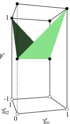
sinceγ∗11=1−γ∗01 andγ∗12=1−γ∗02; its projection in(γ∗01,γ∗02,ϕ∗)space is given in Figure 7. The 6 •’s are the vertices which are not removed after assuming monotonicity and the 6 ◦’s, which correspond to dashes in Figure 6, are the vertices which are removed. Figure 7 clearly demonstrates that the constraints without monotonicity are trivial whereas those with it are not.
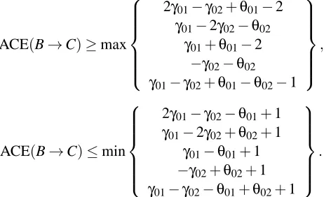
To determine the effect of the monotonicity assumption on the constraints and bounds with (~γ,~θ)in §5, the same mapping is used as in the derivation of the bivariate bounds onαbut applied to the restricted
T
and ˆT
formed by removing the appropriate vertices. The falsifiable constraints obtained areθ01−θ02≥ |γ01−γ02|(equivalent to Equation (7)) and the causal boundsACE(B→C)≥max
2γ01−γ02+θ01−2 γ01−2γ02−θ02
γ01+θ01−2 −γ02−θ02 γ01−γ02+θ01−θ02−1
,
ACE(B→C)≤min
2γ01−γ02−θ01+1 γ01−2γ02+θ02+1
γ01−θ01+1 −γ02+θ02+1 γ01−γ02−θ01+θ02+1
.
mono-1
0 γ∗
01 1
γ∗ 02 -1 1
ϕ∗
Figure 7: The extreme vertices which satisfy monotonicity are the 6•’s, the 6◦’s are those which do not. The convex hull of the transformed polytope for the IV model with the mono-tonicity assumption is the region above the shaded surface and without the monomono-tonicity assumption is the entire cuboid.
tonicity are recovered. The bounds correspond to results in Robins (1989) and Manski (1990). Thus the IV model with monotonicity, introduced in this section, is empirically and computationally in-distinguishable from the IV model with ‘no defiers’ considered in Example 1 and Angrist et al. (1996).
9. Data Analysis
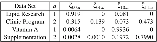
The relative frequencies for two data sets are given in Table 1 and described below.
9.1 Lipid Research Clinics Coronary Data
Consider the Lipid Research Coronary Primary Prevention Trial (Lipid Research Clinic Program, 1984), which was analysed by Efron and Feldman (1991) and Balke and Pearl (1997). Subjects were randomized into two groups, 172 men were given the placebo and 165 were given the treatment, and the subjects’ cholesterol levels were measured. There was partial compliance with the treatment assigned.
9.2 Vitamin A Supplementation
Data Set a ζˆ00.a ζˆ01.a ζˆ10.a ζˆ11.a
Lipid Research 1 0.919 0 0.081 0 Clinic Program 2 0.315 0.139 0.073 0.473 Vitamin A 1 0.0064 0 0.9936 0 Supplementation 2 0.0028 0.0010 0.1972 0.7990
Table 1: Relative frequencies derived from the data sets in Lipid Research Clinic Program (1984) and Sommer and Zeger (1991).
In these trials, the relative frequencies are the maximum likelihood estimates of the parameters
~v. Bounds on ACE(B→C)are computed under various assumptions from the data in Table 1 and are given in Table 2. Sampling uncertainty is ignored here but can be properly considered using techniques described in Ramsahai and Lauritzen (2011).
Study Assumptions Lower bound Upper bound
Lipid IV model 0.392 0.780
Research IV, no randomization -0.145 0.855 Clinic IV, partial exclusion restriction (ε=0.5) 0.050 0.855 Program IV, monotonicity 0.392 0.780
IV model -0.1946 0.0054
Vitamin A IV, no randomization -0.587 0.413 Supplement. IV, partial exclusion restriction (ε=0.5) -0.392 0.212 IV, monotonicity -0.1946 0.0054
Table 2: Causal bounds on ACE(B→C) computed from Lipid Research Clinic Program (1984) and Vitamin A Supplementation Study under various assumptions.
From Table 2, the imposition of the monotonicity assumption has no effect and is unnecessary for these data sets. However the randomized treatment assignment is important since the bounds computed without randomization are very wide and not much can be inferred about the causal effect. Even though the bounds are much wider for the Lipid Research Clinic Program (1984) data, under the partial exclusion restriction withε=0.5, it can still be deduced that there is a positive causal effect.
10. Discussion
The methods given here are applied while relaxing various assumptions that are often used in the deterministic counterfactual IV model. By removing the assumption that there are latent determin-istic mechanisms, it is shown that the same bounds and constraints are obtained and that the models are empirically equivalent §3. The results for models which relax the randomization and exclusion restriction assumptions are valuable for sensitivity analyses. They are also useful for applications in which some of the assumptions in the IV model are known to be false.
compute bounds and constraints as a function ofεbut that would be worthy of future investigation. Such results would show how the bounds vary withεand whether the data places any restrictions on the possible values ofε.
The ideas discussed can be extended to other models involving conditional independence since it is the factorization of the probability distribution which determines the algebraic structure of the polytope representing the model. The model must satisfy the condition that the observable distributions lie in the convex hull of the latent distribution. The vector of parameters P(
X
)always lies in the convex hull of P(X
|U)but there is no guarantee that the factorisation of P(X
|U)produces any non-trivial constraints, whereX
and U are collections of observed and unobserved variables respectively. However there may be non-trivial constraints on conditional probabilities derived from P(X
).Acknowledgments
Steffen Lauritzen has been very helpful with this research. Detailed comments from anonymous referees have helped improve the paper.
Appendix A. Notation
The symbols used throughout are listed below.
ζ∗
cb.a=P(C=c,B=b|A=a,U),
η∗
b=P(C=1|B=b,U),
δ∗
a=P(B=1|A=a,U),
α=P(C=1||B=1)−P(C=1||B=0),
α∗=P(C=1|B=1,U)−P(C=1|B=0,U),
γ∗
ca=P(C=c|A=a,U),
θ∗
ba=P(B=b|A=a,U).
The symbols with∗are functions of U and the corresponding symbols without∗ are the marginals over U .
Appendix B. Equivalence of Convex Hulls
Theorem 1
H
=H
ˆ .Proof Following Dawid (2003), since ˆ
V
⊆V
and ˆH
is the minimal convex set containing ˆV
then ˆH
⊆H
.Let m(~v∗)be an affine function, that is a linear function plus a constant, of~v∗, which returns a scalar, for~v∗∈
V
. A closed half space in [0,1]8 that contains~v is defined by an affine function inequality m(~v∗)≥0 or m{Ξ(~τ∗)} ≥0 for~τ∗∈T
. From Equations (3) and (2), m{Ξ(~τ∗)} is a monotonic function of any single component of~τ∗ when the other three are fixed. Therefore the minimum of m{Ξ(~τ∗)}overT
is attained for some~τ∗∈T
ˆ. ThereforeThis means that any half space containing ˆ
V
also containsV
. Since ˆH
is the intersection of all half spaces containing ˆV
thenV
⊆H
ˆ . Since ˆH
is convex andH
is the minimal convex set containingV
thenH
⊆H
ˆ .Appendix C. Causal Bounds for Binary Instrumental Variable Model
For the binary IV model of Figure 2 (right), bounds onαin terms ofζcb.aare
α≥max
ζ00.1+ζ11.2−1 ζ11.1+ζ00.2−1
−ζ01.1−ζ10.1+ζ11.1−ζ10.2−ζ11.2 −ζ10.1−ζ11.1−ζ01.2−ζ10.2+ζ11.2
−ζ01.1−ζ10.1 −ζ01.2−ζ10.2
−ζ00.1−ζ01.1+ζ00.2−ζ01.2−ζ10.2 ζ00.1−ζ01.1−ζ10.1−ζ00.2−ζ01.2
, and
α≤min
1−ζ10.1−ζ01.2 1−ζ01.1−ζ10.2
ζ00.1−ζ01.1+ζ11.1+ζ00.2+ζ01.2 ζ00.1+ζ01.1−ζ01.2+ζ00.2+ζ11.2
ζ00.1+ζ11.1 ζ00.2+ζ11.2
ζ10.1+ζ11.1+ζ00.2+ζ11.2−ζ10.2 ζ00.1−ζ10.1+ζ11.1+ζ10.2+ζ11.2
.
For the binary IV model of Figure 2 (right), bounds onαin terms ofγcaandθbaare
α≥max
2γ01−γ02+2θ01−3 γ01+θ01−2 γ02+θ02−2 −γ01+2γ02+2θ02−3 −γ01+γ02−θ01+θ02−1
−γ01−θ01 −γ02−θ02 γ01−2γ02−2θ02 −2γ01+γ02−2θ01 γ01−γ02+θ01−θ02−1
and
α≤min
−2γ01+γ02+2θ01+1 γ01−2γ02+2θ02+1 2γ01−γ02−2θ01+2 −γ01+2γ02−2θ02+2 γ01−γ02−θ01+θ02+1
−γ02+θ02+1 γ01−θ01+1 γ02−θ02+1 −γ01+θ01+1 −γ01+γ02+θ01−θ02+1
.
Appendix D. Causal Bounds for Instrumental Variable Model Without Exclusion Restriction
For the binary IV model without the exclusion restriction in §7, forε=0.5, the following bounds are obtained for a=1,2
2{E(C|A=a,FB=1)
−E(C|A=a,FB=0)} ≥max
−2ζ01.a−2ζ10.a
−ζ01.a−2ζ10.a+ζ11.a+ζ00.a′−ζ10.a′−1
2ζ00.a−2−ζ01.a′+ζ11.a′
−3ζ01.a−2ζ10.a−ζ11.a−ζ01.a′+ζ11.a′
−3ζ01.a−2ζ10.a+ζ11.a−2ζ10.a′−2ζ11.a′
−ζ01.a−2ζ10.a−3ζ11.a−3ζ01.a′−2ζ10.a′+ζ11.a′
2ζ11.a+ζ00.a′−ζ10.a′−2
−2ζ01.a′−2ζ10.a′−1
−3ζ01.a−4ζ10.a−ζ11.a+2ζ10.a′+2ζ11.a′−1
ζ01.a+2ζ10.a+3ζ11.a−3ζ01.a′−4ζ10.a′−ζ11.a′−2
, and
2{E(C|A=a,FB=1)
−E(C|A=a,FB=0)} ≤min
2ζ00.a+2ζ11.a
2−2ζ10.a−ζ01.a′+ζ11.a′
2−ζ01.a−2ζ10.a+ζ11.a−ζ01.a′+ζ11.a′
1+2ζ00.a′+2ζ11.a′
2−2ζ01.a+ζ00.a′−ζ10.a′
3ζ00.a−ζ10.a+2ζ11.a+2ζ10.a′+2ζ11.a′
3−3ζ01.a−2ζ10.a−ζ11.a+ζ00.a′−ζ10.a′
4−3ζ01.a−2ζ10.a+ζ11.a−2ζ10.a′−2ζ11.a′
4+ζ01.a−2ζ10.a−ζ11.a−3ζ01.a′−2ζ10.a′+ζ11.a′
4−ζ01.a+2ζ10.a+ζ11.a−3ζ01.a′−4ζ10.a′−ζ11.a′
.
where a′=2 if a=1 and a′=1 if a=2.
References
J. D. Angrist, G. W. Imbens and D. B. Rubin. Identification of causal effects using instrumental variables. J. Am. Statist. Assoc., 91(434):444–455, 1996.
A. Balke. Probabilistic counterfactuals: semantics, computation and applications. PhD Dissertation, University of California, Los Angeles, 1995.
A. Balke and J. Pearl. Non-parametric bounds on causal effects from partial compliance data. Technical Report R-199, Computer Science Department, University of California, Los Angeles, 1993.
A. Balke and J. Pearl. Bounds on treatment effects from studies with imperfect compliance. Journal of the American Statistical Association, 92(439):1171–1176, 1997.
Z. Cai, M. Kuroki, J. Pearl and J. Tian. Bounds on direct effects in the presence of confounded intermediate variables. Biometrics, 64(3):695–701, 2008.
T. Christof and A. Loebel. PORTA. Available online at URL: http://www.iwr.uni-heidelberg.de/groups/comopt/software/PORTA/, 1998.
A. P. Dawid. Conditional independence in statistical theory (with discussion). Journal of the Royal Statisitical Society, Ser. B, 41(1):1–31, 1979.
A. P. Dawid. Causal inference without counterfactuals (with discussion). Journal of the American Statistical Association, 95(450):407–448, 2000.
A. P. Dawid. Influence diagrams for causal modelling and inference. International Statistical Review, 70(2):161–189, 2002.
A. P. Dawid. Causal inference using influence diagrams: the problem of partial compliance. In P. J. Green, N. L. Hjort and S. Richardson, editors, Highly Structured Stochastic Systems, Oxford University Press, New York, 2003.
A. P. Dawid and V. Didelez. Identifying the consequences of dynamic treatment strategies: a deci-sion theoretic overview. Statistics Surveys, 4:184–231, 2010.
V. Didelez, A. P. Dawid and S. Geneletti. Direct and indirect effects of sequential treatments. In Proceedings of the Twenty Second Annual Conference on Uncertainty in Artificial Intelligence, pages 138–146, AUAI Press, Arlington, Virginia, 2006.
V. Didelez and N. Sheehan. Mendelian randomisation as an instrumental variable approach to causal inference. Statistical Methods in Medical Research, 16(4):309–330, 2007.
J. Durbin. Errors in variables. Review of the International Statistical Institute, 22(1):23–32, 1954.
B. Efron and D. Feldman. Compliance as an explanatory variable in clinical trials. Journal of the American Statistical Association, 86(413):9–26, 1991.
D. Geiger and C. Meek. Graphical models and exponential families. In Proceedings of the Four-teenth Annual Conference on Uncertainty in Artificial Intelligence, pages 156–165, Morgan Kauf-mann, San Francisco, California, 1998.
S. Geneletti. Identifying direct and indirect effects in a non-counterfactual framework. Journal of the Royal Statistical Society, Ser. B, 69(2):199–215, 2007.
M. Goldszmidt and J. Pearl. Rank based systems: a simple approach to belief revision, belief update, and reasoning about evidence and actions. In Proceedings of the Third International Conference on Knowledge Representation and Reasoning, Morgan Kaufmann, San Mateo, California, 1992.
D. Heckerman and R. Shachter. Decision theoretic foundations for causal reasoning. Journal of Artificial Intelligence Research, 3:405–430, 1995.
K. Hirano, G. W. Imbens, D. B. Rubin and X.-H. Zhou. Assessing the effect of an influenza vaccine in an encouragement design. Biostatistics, 1(1):69–88, 2000.
G. W. Imbens and J. D. Angrist. Identification and estimation of local average treatment effects. Econometrica, 62(2):467–475, 1994.
C. Kang and J. Tian. Inequality constraints in causal models with hidden variables. In Proceedings of the Twenty Second Annual Conference on Uncertainty in Artificial Intelligence, pages 233– 240, AUAI Press, Arlington, Virginia, 2006.
S. Kaufman, J. S. Kaufman and R. F. MacLehose. Analytic bounds on causal risk difference in directed acyclic graphs involving three observed binary variables. Journal of Statistical Planning and Inference, 139(10):3473–3487, 2009.
S. L. Lauritzen. Graphical models. Oxford University Press, Clarendon, Oxford, UK, 1996.
S. L. Lauritzen. Causal inference from graphical models. In O. E. Barndorff-Nielsen, D. R. Cox and C. Kl¨uppelberg, editors, Complex Stochastic Systems, CRC Press, London, 2001.
S. L. Lauritzen. Discussion on causality. Scandinavian Journal of Statistics, 31(2):189–201, 2004.
S. L. Lauritzen, A. P. Dawid, B. N. Larsen and H. G. Leimer. Independence properties of directed Markov fields. Networks, 20(5):491–505, 1990.
Lipid Research Clinic Program. The lipid research clinics coronary primary prevention trial results, part I and II. Journal of the American Medical Association, 251(3):351–374, 1984.
C. F. Manski. Non-parametric bounds on treatment effects. American Economic Review, Papers and Proceedings, 80(2):319–323, 1990.
J. Pearl. Comment: graphical models, causality and interventions. Statistical Science, 8(3):266– 269, 1993.
J. Pearl. Direct and indirect effects. In Proceedings of the Seventeenth Annual Conference on Un-certainty in Artificial Intelligence, pages 411–420, Morgan Kaufmann, San Francisco, California, 2001.
R. R. Ramsahai. Causal bounds and instruments. In Proceedings of the Twenty Third Annual Con-ference on Uncertainty in Artificial Intelligence, pages 310–317, AUAI Press, Corvallis, Oregon, 2007.
R. R. Ramsahai and S. L. Lauritzen. Likelihood analysis of the binary instrumental variable model. Biometrika, 98(4):987–994, 2011.
T. S. Richardson and J. M. Robins. Analysis of the binary instrumental variable model. In R. Dechter, H. Geffner and J. Y. Halpern, editors, Heuristics, probability and causality: a tribute to Judea Pearl, College Publications, UK, 2010.
J. M. Robins. The analysis of randomized and non-randomized AIDS treatment trials using a new approach to causal inference in logitudinal studies. In L. Sechrest, H. Freeman and A. Mulley, editors, Health Service Research Methodology: a Focus on AIDS, U.S. Public Health Service, Washington D.C., 1989.
J.M. Robins and S. Greenland. Identifiability and exchangeability for direct and indirect effects. Epidemiology, 3(2):143–155, 1992.
J. M. Robins and T. S. Richardson. Alternative graphical causal models and the identification of direct effects. In P. Shrout, editor, Causality and Psychopathology: Finding the Determinants of Disorders and Their Cures, Oxford University Press, 2010.
D. B. Rubin. Estimating causal effects of treatments in randomized and nonrandomized studies. Journal of Educational Psychology, 66(5):688–701, 1974.
B. E. Shepherd, P. B. Gilbert, Y. Jemiai and A. Rotnitzky. Sensitivity analyses comparing outcomes only existing in a subset selected post randomization, conditional on covariates, with application to HIV vaccine trial. Biometrics, 62(2):332–342, 2006.
A. Sj¨olander. Bounds on natural direct effects in the presence of confounded intermediate variables. Statistics in Medicine, 28(4):558–571, 2009.
A. Sommer and S. L. Zeger. On estimating efficacy from clinical trials. Statistics in Medicine, 10(1):45–52, 1991.
P. Spirtes, C. Glymour and R. Scheines. Causation, Prediction and Search. Springer-Verlag, New York, 1993.
R. H. Strotz and H. O. A. Wold. Recursive vs non-recursive systems: an attempt at synthesis (part I of a triptych on causal chain systems). Econometrica, 28(2):417–427, 1960.