Grinding Chatter Detection and Identification Based on BEMD and LSSVM

ORIGINAL ARTICLE

Grinding Chatter Detection

and Identification Based on BEMD and LSSVM

Huan‑Guo Chen

_{, Jian‑Yang Shen}

_{, Wen‑Hua Chen}

_{, Chun‑Shao Huang}

_{, Yong‑Yu Yi}

_{and Jia‑Cheng Qian}

Abstract

Grinding chatter is a self‑induced vibration which is unfavorable to precision machining processes. This paper proposes a forecasting method for grinding state identification based on bivarition empirical mode decomposition (BEMD) and least squares support vector machine (LSSVM), which allows the monitoring of grinding chatter over time. BEMD is a promising technique in signal processing research which involves the decomposition of two‑dimen‑ sional signals into a series of bivarition intrinsic mode functions (BIMFs). BEMD and the extraction criterion of its true BIMFs are investigated by processing a complex‑value simulation chatter signal. Then the feature vectors which are employed as an amplification for the chatter premonition are discussed. Furthermore, the methodology is tested and validated by experimental data collected from a CNC guideway grinder KD4020X16 in Hangzhou Hangji Machine Tool Co., Ltd. The results illustrate that the BEMD is a superior method in terms of processing non‑stationary and nonlinear signals. Meanwhile, the peak to peak, real‑time standard deviation and instantaneous energy are proven to be effec‑ tive feature vectors which reflect the different grinding states. Finally, a LSSVM model is established for grinding status classification based on feature vectors, giving a prediction accuracy rate of 96%.

Keywords: Grinding chatter, BEMD and LSSVM, Complex‑value chatter signal, Feature vector, Grinding status classification

© The Author(s) 2019. This article is distributed under the terms of the Creative Commons Attribution 4.0 International License (http://creat iveco mmons .org/licen ses/by/4.0/), which permits unrestricted use, distribution, and reproduction in any medium, provided you give appropriate credit to the original author(s) and the source, provide a link to the Creative Commons license, and indicate if changes were made.

1 Introduction

Grinding is an abrasive machining process which is widely used in modern manufacturing practice to pro-duce high surface quality and close tolerance [1–4]. Particularly with the increasing mature of ultra-high speed grinding, its advantages are further improved, that providing convenient conditions for development of aerospace technology, transportation, military and other industries [5, 6]. However, grinding chatter is one of the most unfavorable dynamic phenomena in grind-ing operations includgrind-ing regenerative chatter, frictional chatter and mode coupling chatter. In practice, grinding chatter has negative impacts on the ultimate geometri-cal workpiece accuracy, surface quality and productivity of machinery. Moreover, it leads to increased wheel wear and adds time and costs to manufacturing [7, 8]. Many

theories have been proposed and experiments carried out to discover exactly what mechanism underlies grind-ing chatter, with the aim of developgrind-ing reliable suppres-sion methods subsequently [9].

At present, only a few methods for chatter detec-tion have been successfully and practically applied in industry. It is common for trained machine operators to identify the appearance of chatter through experience or observation, meaning that corresponding measure-ments are not taken at the time that resulting in irrepa-rable loss for the industry. Signal processing techniques and appropriate feature vectors are very important for chatter detection. In the past few decades, either non-linear time series modeling [10] or spectral analysis [11, 12] has been applied for chatter detection. Additionally, Tansel et  al. [13], adopted s-transformation to extract the damping index, making a very descriptive feature of chatter available for inspection in turning operations. Yao et al. [14], presented a two-dimensional feature vec-tor for chatter detection based on the standard deviation of wavelet transforms in drilling machining which had

Open Access

*Correspondence: [email protected]

1 _{Zhejiang Province’s Key Laboratory of Reliability Technology}

an advantageous identification time. In another study, Gradisek et al. [15] used the coarse-grained entropy rate as a chatter index in grinding and turning, as its value exhibits a drastic drop at the onset of chatter.

It is important to note that the signal processing meth-ods proposed above were mostly based on the theory of Fourier transformation and that these traditional methods are not applicable to processing grinding sig-nals (which are almost non-stationary and nonlinear). They can only detect chatter if it is already in an almost fully developed stage and easily to extract spurious fre-quency and error information from chatter signals. In order to highly meet the demand of real-world produc-tion, it is necessary to detect the onset of chatter before chatter marks have been made on the workpiece. Given this requirement, Rilling et  al. [16] proposed a novel method called the bivarition empirical mode decomposi-tion (BEMD). In the third session of the HHT (Hilbert– Huang Transform) International conference, BEMD was successfully applied to the monitoring of wind turbine conditions and displayed its feasibility as a method to determine weak features and integrate information from non-stationary and nonlinear signals [17].

The author of this paper also has made a compari-son between EMD and BEMD in extracting features for grinding chatter signals to show the advanced perfor-mance of BEMD, that the paper is accepted by the 2016 11th International Conference on Reliability, Main-tainability and Safety (ICRMS’ 2016). Thus will not be repeated in details here and just give out some brief conclusions about the distinctions between EMD and BEMD: (1) EMD is initially applied to a one-dimen-sional signal and extracts zero-mean oscillating compo-nents, whereas BEMD is applied to a bivariate signal and extracts zero-mean rotating components; (2) BEMD has calculation efficiency due to process complex-value sig-nals simultaneously and only compute the upper enve-lope using the maximum points, while EMD can only decompose signals one-by-one and has to obtain both upper and lower envelopes by connecting the extreme points; (3) The number of IMFs derived from signals by EMD are different, and can’t reveal any synchronous characteristics and phase shifting, nor can EMD extract an information fusion function. While the number of IMFs by BEMD is the same, it can extract an information fusion function well and preserve phase differences; (4) BEMD has facilitates the establishment of purified shaft vibration orbits and fully guarantees the correctness of results, which EMD cannot.

Additionally, there are several smart classifiers essential for grinding state identification, such as artificial neural network (ANN) [18, 19], fuzzy logic and support vector machines (SVM). Li et al. [20] used multilayer perceptron

ANN to distinguish the tool breakage and cutting chatter. According to the trend of signal in time domain. Bedi-aga, et al. [21] established the fuzzy logical rule to ana-lyze stability of cutting system. Moreover, Jiang et al. [22] adopted multi-class SVM to identify and classify cutting states that accuracy rate reached 95%. The ANN usually suffers from the problem of intrinsic defeats such as slow study speed, multiple local minima and over-fitting. Also, the prediction ability of fuzzy logic is inaccurate and its theory is still imperfect. SVM overcomes these deficien-cies by using the structural risk minimization principle to enhance extensive ability and it also stresses the study of statistical learning rules with a small sample. In order to further improve the learning speed [23]. Suykens pro-posed a modified version of SVM, i.e. the least squares SVM (LSSVM). In the LSSVM, the non-sensitive loss function is replaced by a quadratic loss function and the inequality constraints are replaced by equality con-straints. Through constructing a loss function, the quad-ratic programming problem is translated into solving linear equation group problems, which simplifies the complexity of calculation [24, 25].

The advantages of BEMD and LSSVM are combined in this paper for detecting and identifying grinding chatter. Section two gives a brief review of BEMD and LSSVM, as well as the extraction criterion of true BIMFs. Moreo-ver, the peak to peak, real-time standard deviation and instantaneous energy are presented as feature vectors for the grinding chatter. In section three, a simulation chat-ter signal is constructed and then processed by BEMD. Afterwards, peak to peak, real-time standard deviation and instantaneous energy are extracted from BIMFs. In section four, the benefits of the proposed method are further validated experimentally by processing grinding signals which are derived from the grinder KD4020X16, and then a LSSVM model is established to predict the grinding state. Finally, conclusions are presented in sec-tion five, which also gives new direcsec-tions for future work.

2 BEMD and LSSVM

2.1 A Brief Review of BEMD

2.1.1 Algorithm of BEMD

(1) The number of extrema and zeros must be equal or different at most by one.

(2) The mean value of the envelope at any point defined by the local maximum points and the envelope as defined by the local minima must be zero.

The fundamental sifting process of BEMD can be depicted as follows.

S1 Select a bivariate signal s(t)=x(t)+iy(t) and a set

of projection directions: ϕk=2kπ/N, 1≤k≤N S2 For 1≤k≤N.

S21 Project the signal s(t) on directions ϕk :

S22 Extract all partial maximum points of pϕk(t):

{(t_ik,pk_i)} , where i indicates number of individual

maxima.

S23 Interpolate the set of points

t_ik,pk_i exp(iϕk)

by cubic spline interpolation to obtain the partial envelope curve in direction ϕ_k , namely, eϕk(t).

S3 Calculate the mean of all envelop curves:

S4 Subtract the mean m¯(t) from s(t) to obtain g(t):

S5 Examine if g(t) is a BIMF:

S51 If not, replace s(t) by g(t) and repeat the procedure

from step S2 until g(t) is a BIMF.

S52 If it is, record the obtained BIMF and repeat the

procedure from step S2 on the residual signal g(t).

As well as referring to the sifting process of BEMD, the s(t) can be expressed by the procedure:

where gm(t) denotes the mth complex-valued BIMF and rn(t) denotes the residue.

2.1.2 Extraction Criteria of True BIMFs

It is worth noting that the above-generated BIMFs basi-cally incorporate two components: true BIMFs and spuri-ous BIMFs. These spurispuri-ous BIMFs cannot exactly reflect the vibration peculiarities of grinding systems in a physi-cal sense and this seriously interferes with the researchers’

(1) pϕk =Re[s(t)exp(−iϕk)].

(2) ¯

m(t)= 1

N

N

k=1

eϕk(t),

(3) g(t)=s(t)− ¯m(t).

(4) s(t)=

n

m=1

gm(t)+rn(t),

efforts to extract the feature vectors from signals and elimi-nate the mechanism faults of grinders. In general, the gen-eration of spurious BIMFs are summarized by the following factors: (1) the definition of BIMFs is only based on numer-ical analysis, without referring to its physnumer-ical significance; (2) the stopping criterion of the sifting process results in an excessive decomposition phenomenon; (3) end effect which can lead to serious deviation from the actual features of the signal is not fully eliminated; (4) either white noise or pulse interference which is superimposed on the vibra-tion signal may produce high frequency spurious compo-nents. Considering that the majority of people rely heavily on their experience to estimate the authenticity of BIMFs, this is not conducive to facilitating the expansion of the BEMD method. It is therefore necessary to use an efficient and reliable method to identify and eliminate the spurious BIMFs, a procedure which is of great importance to the extraction of the actual vibration mode and corresponding features of the time-frequency domain.

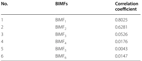
As the BIMFs are recognized as the orthogonal expres-sion of the signal, the true BIMFs will have a higher correla-tion with the original signal compared to the spurious BIMFs. Therefore, it is reasonable to employ the correlation coefficient as a measurement index to remove the spurious components and then classify it as part of a residual [28]. The specific sifting process could be described as in Table 1, if the correlation coefficient of each complex-value BIMF

ζm=

ζ1

m ×

ζ2

m

,(m=1, 2,. . .,n) , has been obtained

(where, ζ_m1 and ζ_m2 denote the correlation coefficient of the

real and imaginary parts of BIMFs, respectively).

The η in Table 1 is a fixed threshold that is generally adopted as a ratio of the maximum correlation coefficient, where δ is a ratio coefficient larger than 1:

2.2 Brief Review of LSSVM

The LSSVM is an improved algorithm based upon standard SVM that a two-norm is taken with equality instead of inequality constraints so as to obtain a linear set of equations instead of a quadratic programming problem in the dual space [29, 30]. It shows specific powerful capability in processing small sample, non-linear and high-dimension pattern. The formulation of LSSVM can be described as follows:

(5)

η=max(ζm/δ), m=1, 2,. . .,n.

Table 1 Extraction criterion of  true BIMFs based on correlation coefficient

If ζm≥η,

Reserve the mth _{BIMF gm;} Else

(1) Using a training set of the data points D= {(xi,yi)|i=1, 2,. . .,n} , where xi ∈Rn is the

ith input data, and yi∈ {−1,+1} is the output class.

(2) The regression function in high-dimensional space is constructed:

where ω is the weight vector, ϕ(x) is a nonlinear

function that maps the input data x into a

low-dimension space and b is the bias parameter.

(3) According to the structural risk minimization

prin-ciple, the optimal ω and b can be obtained by

mini-mizing the following function:

where C is the penalty coefficient to balance the

structural risk and experience risk and ε_i is the slack

variable.

(4) The Lagrange function can be constructed to solve the optimization problem:

where α_i represent Lagrange multipliers that can

be either positive or negative values. Eq. (8) can be

changed to the following equivalent equations:

(5) Eliminating ω and ε_i and expressing in matrix form

gives:

where

(6)

y(x)=ω·ϕ(x)+b,

(7)

min

ω,b,εJ(

ω,ε)= 1

2�ω�

2₊C

2

n

i=1 ε2_i,

s.t.yi=ω·ϕ(xi)+b+εi,

(8)

L(ω,b,ε,α)=J(ω,ε)− n

i=1

αi(ω·ϕ(xi)+b+εi−yi),

(9)                ∂L

∂ω =0⇒ω− n

�

i=1

αiϕ(xi)=0,

∂L ∂b=0⇒

n

�

i=1 α_i=0,

∂L

∂εi =0⇒Cεi−αi =0, ∂L

∂αi =0⇒ω·ϕ(xi)+b+εi−yi =0.

(10)

0 eT

e i,j+C−1I

b α = 0 y ,

e= [1, 1,. . ., 1]T_n,

y= [y1,y2,. . .,yn],

α= [α1,α2,. . .,α_n]T,

i,j=(xi)×(xj)=K(xi,xj) is the kernel function.

The commonly used kernel functions are listed as

follows [31, 32].

Polynomial kernel function:

RBF kernel function:

Sigmoid kernel function:

(6) Lastly, the linear model for function estimation is achieved after the optimization problem is solved:

2.3 Chatter Feature Vectors Extraction

Numerous experiments have shown that the amplitude of the vibration signal fluctuates within a certain range when the grinder is in a stable grinding state, while the amplitude substantially increases when in a transition state. It later becomes steady again when the grinder is in a chatter state; Therefore, early grinding chatter can be preliminary detected by comparing changes in the time-domain statistical parameters of the signal. In this paper, the peak to peak (pp), real-time standard deviation (Rsd) and instantaneous energy (IE) are conceived as ideal fea-ture vectors that can detect and identify the chatter.

The peak to peak represents the difference between the maximum and minimum values of the signal, which is recognized as the most intuitive indicator for amplitude change in the signal [33]:

where N represents the sampling points.

The real-time standard deviation indicates the devia-tion degree from the mean chatter signal, which in a sense reflects the oscillation trend [34]. Rsd can be described as:

(11) K(xi,xj)=((xi,xj)+θ )d, d=1, 2,. . .

(12)

K(xi,xj)=exp

−x_i−x_j 2 σ2 . (13) K(xi,xj)=tanh(υ(xi,xj)+c).

(14) y(x)=

n

i=1

α_iK(xi,xj)+b.

(15) pp= |{xi}|max− |{xi}|min, i=1, 2,. . .,N,

(16)

Rsd2=1

n

n

i=1

(|xi| − ¯x)2

=1

n

n

i=1

x_i2−1

n

n

i=1

xi

=

x2₁

n − x1 n +

x2₂

n − x2 n + · · · +

x_n2

n −

xn

n

where x¯ represents the mean of the signal.

In practice, any internal fluctuation may result in a vibration of instantaneous energy, which means that the change in instantaneous energy has a direct relation to

abnormal system operation [35]. Thus, instantaneous

energy can be defined as follows:

where αi and ψi represent the instantaneous amplitude of

the real and imaginary parts of signal respectively [36]. Using these definitions, the pp, Rsd and IE of each BIMF can be monitored every second, achieving initially detecting grinding chatter in real time.

3 Application of BEMD to Simulate Chatter Signal

3.1 Construction of a Simulation Chatter Signal

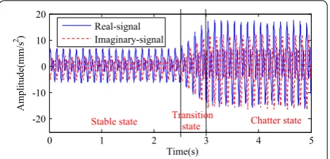
In order to evaluate whether BEMD could be a reliable technique employed for grinding chatter detection, a simulation of a complex-value chatter signal s(t) was con-structed according to the mechanism of chatter and char-acteristics of the time-frequency domain:

where

It is clearly seen that the real and imaginary parts of sig-nal s(t) are composed of two sine signals and white noise, respectively, and that the frequency components of both are 50 rad/s and 100 rad/s. Additionally, the phase of the imaginary parts of signal is shifted by 0.08 rad and 0.024 rad. The output is a harmonic vibration signal which simulates the stable grinding process when t ≤ 2.5 s. The output is the harmonic vibration signal multiplied with a slant sign also as to simulate the grinding chatter when 2.5 < t ≤ 3  s. Moreover, the output is the original har-monic vibration signal multiplied by gain coefficients in order to simulate the stable chatter status when 3 < t ≤ 5 s.

The chatter signal is shown in Figure 1. The blue solid lines represent the real part of signal while the red dash lines indicate the imaginary part. It is clearly seen that the amplitude of the signal is small in a stable grind-ing process, while the amplitude significantly increases

(17)

IE = 1

2 α

2 i +jψi2

, j=

√

−1,i=1, 2,. . .,N,

(18)

s(t)= 

 

 

x(t)+c1(t)+i(y(t)+c2(t)), 0≤t≤2.5, (x(t)+c1(t))(1+4(t−2.5))+i((y(t)+ · · ·

· · · +c2(t))(1+5(t−2.5)), 2.5<t≤3, 2.5(x(t)+c1(t))+i3(y(t)+c2(t)), 3<t≤5,

(19)

x(t)=3 sin(50t)+4 sin(100t)+0.4,

y(t)=2 sin(50t+4)+3 sin(100t+2.4)−0.2, c1(t)=1.5rand(2001, 1)−0.75,

c2(t)=rand(2001, 1)−0.5.

after 2.5 s, then after 3 s the amplitude become steady as the grinder settles into stable chatter. Hence it’s change trend and distribution are similar to experimental chatter images in Refs. [14, 37], that this chatter signal well simu-lates the chatter process.

3.2 Application of BEMD

Decomposing this chatter signal using BEMD sets 64 projection directions and 10 iterations, generating the BIMFs shown in Figure 2. The blue solid lines represent the real part of the BIMFs while the red dash lines indi-cate the imaginary part.

From Figure 2, it is seen that the simulation complex-value chatter signal is decomposed into 6 BIMFs and a residue, which can significantly facilitate the establish-ment of a pure vibration orbit and fully guarantees the correctness of the established result. The extraction cri-terion of true BIMF introduced in Section 2.1.2 is then applied to the decomposed BIMFs and the correlation coefficients of the BIMFs are shown in Table 2.

Compared with the data in Table 2, only the first two BIMFs, which have a relatively high correlation with orig-inal signals, should be reserved. The other four BIMFs have to be removed and classified as a part of the resid-ual. The true BIMFs which are derived from simulation chatter signals are shown in Figure 3, where the real parts of BIMFs are plotted as blue solid lines and the imaginary parts are plotted as red-dashed lines.

In Figure 3, it is clearly seen that there is mutual dependence between the real and imaginary part of the true BIMFs (i.e., BIMF1 and BIMF2) and that the por-tions where components are rotating can be identified by a constant phase shift. The cross-correlation function (CCF) of each true BIMF could therefore be obtained and then the phase parameters could be estimated from the CCF [38], as shown in Figure 4. Moreover, the ampli-tude and the frequency components of the chatter signal which are initially set in the previous signal also could be revealed by carrying out the Hilbert transformation on the true BIMFs, as shown in Figure 5, where the marginal

0 1 2 3 4 5

-20 -10 0 10 20

Real-signal Imaginary-signal

Chatter state Stable state Transition _state

Time(s)

Amplitude(mm/s

2)

spectrum of real part of signal is plotted as blue solid line and imaginary part of signal is plotted as red-dashed line. The marginal spectrum expresses the amplitude of each frequency in space and represents accumulated ampli-tude in a statistical sense.

According to Figure 4, it is clearly seen that the phase shifting and synchronization information about the real and imaginary parts of the true BIMFs are well pre-served and easily detected. The phase shifting of BIMF1 and BIMF2 is 0.025 rad and 0.08 rad, respectively, which is similar to the phase as described in the simulation sig-nal. From Figure 5, the frequency components of the real and imaginary parts of the signal (8 Hz and 16 Hz) are

0 1 2 3 4 5

-10 0 10

BI

MF

1

0 1 2 3 4 5

-10 0 10

BI

MF

2

0 1 2 3 4 5

-2 0 2

BI

MF

3

0 1 2 3 4 5

-1 0 1

BI

MF

4

0 1 2 3 4 5

-1 0 1

BI

MF

5

0 1 2 3 4 5

-1 0 1

BI

MF

6

0 1 2 3 4 5

-1 0 1

Tr

en

d

Time(s)

Real-BIMF Imaginary-BIMF

Figure 2 The so‑generated BIMFs of simulation chatter signal

Table 2 Correlation coefficient of  BIMFs of  simulation chatter signal

No. BIMFs Correlation

coefficient

1 BIMF₁ 0.8025

2 BIMF2 0.6281

3 BIMF3 0.0526

4 BIMF4 0.0176

5 BIMF5 0.0043

6 BIMF6 0.0147

0 1 2 3 4 5

-10 0 10

BIM

F1

0 1 2 3 4 5

-10 0 10

BIM

F2

0 1 2 3 4 5

-5 0 5

Trend

Time(s)

Real-BIMFs Imaginary-BIMFs

Figure 3 True BIMFs of a simulated chatter signal

0 0.02 0.04 0.06 0.08 0.1

-5 0 5x 10

4

BI

MF

1

0 0.02 0.04 0.06 0.08 0.1

-2 0 2

x 104 Time(s)

BI

MF

2

*

*

Max

Figure 4 CCF and phase parameters of true BIMFs

0 5 10 15 20 25

0 2 4 6 8

Frequency(Hz)

Amplitude(mm/

s

2 )

Real-signal Imaginary-signal

accurately revealed as corresponding with the same fre-quency components, i.e., 50 rad/s and 100 rad/s, as set in the previous signal.

3.3 Extraction of the Chatter Feature Vectors Based on BEMD

Through the decomposition of BEMD and the extraction of true BIMFs, the chatter signal is decomposed into a series of true BIMFs and a residue. Another main objec-tive of this paper is to extract appropriate feature vec-tors of each true BIMF and superpose them respectively to construct synthetic chatter feature vectors for chatter detection and identification. To compare and analyze the chatter feature vectors they should be normalized [39, 40] in order to keep the value between 0 and 1. As described in Section 2.3, the peak to peak, real-time standard devi-ation and instantaneous energy are applied to the chatter signal and the superimposed and normalized feature vec-tors of the BIMFs, along with time, are shown in Figure 6. The pp are plotted as blue solid lines, Rsd are plotted as a black dot lines, while IE are plotted as a red-dashed lines.

In Figure 6, it is clearly seen that all feature vectors in various grinding states exhibit different behaviors and that the amplitude of the feature vectors is almost con-stant in a stable grinding state, while the amplitude drastically increases once the grinder turns into chatter. Moreover, the peak to peak and instantaneous energy fluctuation within a certain range when the grinder is in stable chatter state. The real-time standard deviation continuously increases with time and tends towards sta-bility at the end, making it hard to exactly distinguish the transition state and chatter state. But all in all, it is fea-sible to clearly find out the onset of grinding chatter of great important to take reliable method to suppress the chatter. In summary, the peak to peak, real-time standard deviation and instantaneous energy are significantly dis-tinct and could be used as a predictor for early grinding chatter detection.

4 Grinding Experiments and Application of BEMD and LSSVM

The ultimate purpose of this paper is to distinguish the onset of grinding chatter so that effective methods for chatter suppression can be applied as soon as possible. Therefore, a method based on BEMD and LSSVM is pre-sented to detect and identify the grinding operation state. The process of this method is expressed in Figure 7.

4.1 Grinding Experiments

In order to further validate the feasibility of BEMD in grinding chatter detection, an experimental method was designed to acquire the various vibration states of differ-ent grinding parameters for the CNC guideway grinder KD4020X16 from Hangzhou Hangji Machine Tool Co., Ltd. The IEPE piezoelectric acceleration sensors with a supporting dynamic signal test and analysis system called

0 1 2 3 4 5

0.4 0.6 0.8 1

0 1 2 3 4 5

0.4 0.6 0.8 1

0 1 2 3 4 5

0.4 0.6 0.8 1

Time(s)

Rsd pp IE

Transition state

Chatter state Stable state

BIM

F1

BIM

F2

Synthetic BIM

F

Figure 6 Feature vectors of the BIMFs

Vibration signal acquistion

Signal pre-processing

BEMD-based method for BIMFs BEMD

True BIMFs extraction Hilbert transform

pp Rsd IE

Feature vectors superposing and normalizing

LSSVM

Training

LSSVM modeling

Training

State identifying

TST5912 was used to collect the grinding vibration sig-nal, as shown in Figure 8.

In practice, the grinder is more sensitive to the rota-tional speed, feeding speed and grinding depth of the grinding wheel, which contributes to the unbalance of the grinding vibration. The experiment was therefore car-ried out in following steps:

Firstly, keep the feeding speed of the workpiece and grinding depth of the wheel constant, and then gradually increase the rotational speed.

Secondly, keep the feeding speed and rotational speed constant, and then gradually increase the depth of grinding.

Lastly, keep the rotational speed and depth of grinding constant, and then gradually increase the feeding speed.

The resulting parameters are listed in Table 3.

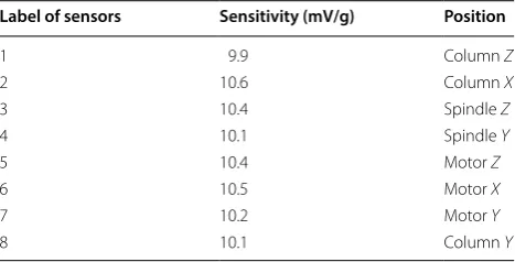
According to the experimental conditions shown in Table  3, eight piezoelectric acceleration sensors are used to test the vibration acceleration signals of grind-ing wheel spindle, motor and machine column in various directions. The position of sensors and corresponding sensitivity are given in Table 4.

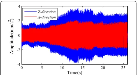
Using the above steps, we collected and recorded cor-responding signals until 80 groups of grinding signals were obtained, where 45 groups were in a stable grinding state, while 35 groups are in a chatter state. It has been proven that chatter of the wheel spindle is more signifi-cantly in the X-direction and Z-direction compared to the Y-direction based upon the practical experience and analysis of a considerable portion of the experimental data. For convenience of presentation, this paper selects parts of the X-direction and Z-direction chatter data to construct a complex-valued signal and then eliminates its noise based on the wavelet transform [41, 42]. The newly constructed complex-valued signal is shown in Figure 9, where the blue solid lines represent the Z-direction part and the red-dashed lines represent the X-direction.

From Figure 9, it is seen that the grinding

chat-ter emerges at about 6‒14  s and the transitional phase remains at almost 8 s. It is clearly seen that the amplitude of the vibration signal rapidly expands when the grinder turns into chatter, then the amplitude becomes steady when the grinder gets into stable chatter. However, the signal vibrates more markedly compared with the stable grinding state.

4.2 Application of BEMD to Experimental Chatter Signals As previously discussed, the BEMD demonstrates its powerful capability in terms of processing the two-dimensional simulation chatter signal and extracting true BIMFs from it. Moreover, the simulation results illustrate the phase information and synchronization between real

and imaginary parts of the BIMFs, which is of signifi-cant value when applying the BEMD method to practical chatter. The BEMD is applicable to decompose the above experimental signal, which sets 64 projection directions at 10 iterations. Then the extraction criterion based on correlation coefficient could be applied to the extracted

Figure 8 CNC guideway grinder KD4020X16 and TST5912 analysis system

Table 3 Grinding parameters

Parameter Value

Grinding wheel material Green silicon carbide Size of wheel (mm × mm) φ600×150

Work‑piece material Gray cast iron 250 Size of workpiece (mm × mm × mm) 3050 × 500 × 500 Rotational speed (r/min) 700 ~ 1100 Feeding speed (m/s) 0.381, 0.254, 0.210 Grinding depth (μm) 5, 10, 15

Table 4 Position of sensors and corresponding sensitivity

Label of sensors Sensitivity (mV/g) Position

1 9.9 Column Z

2 10.6 Column X

3 10.4 Spindle Z

4 10.1 Spindle Y

5 10.4 Motor Z

6 10.5 Motor X

7 10.2 Motor Y

BIMFs so that the correlation coefficients are shown in Table 5.

From Table 5, it is clearly seen that the first four BIMFs which have a relatively high correlation with the original signals should be reserved. The other four BIMFs have to be removed and classified as a part of the residual so the first three BIMFs could be recognized as the true BIMFs, which contain the main frequency components of the signal. The resulting decomposition is shown in Fig-ure 10, where the blue solid lines represent the real part while the red-dashed lines represent the imaginary parts of the BIMFs.

According to Figure 10, it is clearly seen that phase shifting between the real parts and imaginary parts of the true BIMFs are well preserved and detected. Thus, the CCF of each true BIMF could be obtained and then the phase parameter estimated from the CCF, as shown in Table 6.

Then the amplitude and frequency components could be calculated by performing the Hilbert transform on each true BIMF to obtain the marginal spectrum, as shown in Figure 11.

In Figure  11, the marginal spectrum of both the

Z-direction and X-direction shows the same frequency components, which represent about 300  Hz, 580  Hz, 1200  Hz and 1400  Hz. Yet the Z-direction BIMFs have a larger amplitude relative to the X-direction, and signal vibrates more significantly in the Z-direction according to the practical data.

4.3 Chatter Feature Vectors Extraction for the Experimental Signal

Based on the same principle and method, the feature vec-tors could also be extracted from the experimental true BIMFs, where the superimposed and normalized pp, Rsd and IE of real and imaginary parts of the BIMFs, along with time, are shown in Figure 12. The pp of the BIMFs are plotted as blue solid lines, Rsd are plotted as black dot lines, while IE are plotted as red-dashed lines.

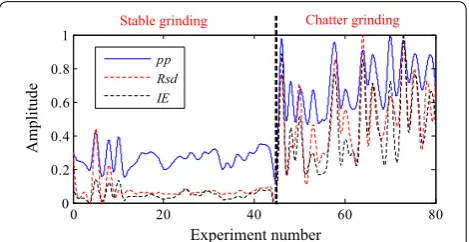
We can see that the behavior of these three feature vec-tors exhibit the same change in regulation as the previous simulation chatter signal in Section 3.3, that it can ini-tially find out the onset time of chatter is nearly 6 s. How-ever, in order to detect and identify the onset of grinding chatter in time, it is very crucial to extract feature vectors during an early stage of its development. Therefore, the chatter feature vectors could be selected at the maximum value of the transition state. Then the feature vectors of the 80 collected grinding signals could be calculated and are shown in Figure 13, after superposing and normaliz-ing, where the first 45 signals are stable grinding and the latter 35 signals are chatter grinding. The pp is plotted as

0 5 10 15 20 25

-4 -2 0 2 4

Time(s)

Z-direction X-direction

Amplitude(mm/s

2 )

Figure 9 Newly constructed complex‑valued signal from experimental data

Table 5 Correlation coefficients of the experimental BIMFs

No. BIMFs Correlation

coefficient

1 BIMF1 0.9656

2 BIMF2 0.0700

3 BIMF3 0.0336

4 BIMF4 0.0156

5 BIMF₅ 0.0032

6 BIMF6 0.0016

7 BIMF7 0.0021

8 BIMF8 0.0014

0 5 10 15 20 25

-4 -2 0 2 4

BIM

F1

0 5 10 15 20 25

-1 0 1

BIM

F2

0 5 10 15 20 25

-0.2 0 0.2

BIM

F3

0 5 10 15 20 25

-0.5 0 0.5

Time(s)

Tren

d

0 5 10 15 20 25

-0.5 0 0.5

BIM

F4

Z-direction X-direction

blue solid line, Rsd is plotted as black dot line, while IE is plotted as red-dashed line.

From Figure 13, it is seen that the pp, Rsd and IE of chatter grinding are increased to a different degree com-pared with stable grinding, that it is considered as the significant characteristic to distinguish the grinding state. Therefore, they are all employed as input data for the LSSVM.

4.4 LSSVM Model Prediction

In accordance with the theory of LSSVM, the model should be established using training samples, which uti-lize feature vectors of 30 stable signals and 25 chatter sig-nals at a random as the training set, with the remaining 15 stable signals and 10 chatter signals used for testing. The training of the LSSVM is performed in Matlab and the process of LSSVM training is actually the learning process from the expert knowledge mentioned in Sec-tion 2.2. Thus, two classifiers should be defined where − 1 represents stable state and + 1 represents chatter state. It is important to choose a suitable kernel function as it can strongly influence the reliability of the LSSVM results. In this paper, after a grid search and cross validation, an RBF kernel function was selected which sets the penalty coefficient C = 1 and ε = 0.1. The grinding parameters, feature vectors, and corresponding prediction results are shown in Table 7.

According to the data in Table 7, the 14 stable grind-ing signals and the other 10 chatter grindgrind-ing signals are exactly identified by the LSSVM model, while the third stable signal is wrong for a chatter signal which is mostly caused by the concentrated load shock. The accuracy of this prediction model is 96%, which could be considered an appropriate model to be applied for chatter detec-tion and identificadetec-tion in the CNC guideway grinder KD4020X16. For convenience of presentation, the pre-diction model can be made into a diagram form, as shown in Figure 14, where the red asterisks and blue cir-cles represent feature vectors of the stable state and chat-ter state, respectively.

It is seen that Figure 14 is the visual expression of the LSSVM prediction model. It is clearly divided into two parts: a stable state area and a chatter state area. More-over, the feature vector distribution of chatter is more extensive than the stable state. Thus, in view of this grinding machine, the feature vectors could be extracted out from the real-time acquired signals by BEMD method, and then tested by this LSSVM model which has

Table 6 Phase and  maximum of  CCF from  each of the experimental BIMFs

Parameter BIMF1 BIMF2 BIMF3 BIMF4

Estimated phase (rad) 0.0562 0.0141 0.0350 0.0562 Maximum of CCF 6517.1 148.55 74.647 7.1760

0 500 1000 1500

0 0.5 1 1.5 2 2.5 3

Frequency(Hz)

Amplitude(mm/

s

2 )×

10

-3 Z-direction X-direction

Figure 11 Marginal spectrum of the Z‑direction signal and

X‑direction signal

0 5 10 15 20 25

-4 -2 0 2 4

Time(s)

0 5 10 15 20 25

0.2 0.4 0.6 0.8 1

Rsd pp IE Real-signal Imag-signal

Stable state

Transition

state Chatter state

Signa

l

Chatter feature

s

Figure 12 The synthetic feature vectors of the signal

0 20 40 60 80

0 0.2 0.4 0.6 0.8 1

pp Rsd IE

Chatter grinding Stable grinding

Amplitude

Experiment number

high accuracy and efficiency. If the feature vectors are in stable area, it means that the grinder is operating well. Otherwise, the grinding machine is suffering from the

chatter, that effective measures should be taken immedi-ately to reduce the damage of chatter. It is also necessary to collect more sample data as training set to improve

Table 7 Prediction results of the LSSVM model

Test No. Input Target Output Result Rotational speed

(r/min) Feeding speed (m/s) Grinding depth (μm)

pp Rsd IE

1 01710 0.4626 1.9618 1 1 Correct 992 0.381 5

2 0.0382 0.0111 0.0353 − 1 − 1 Correct 763 0.381 5

3 0.0830 0.2870 0.2765 − 1 1 Wrong 1034 0.381 5

4 0.0336 0.0113 0.0361 − 1 − 1 Correct 808 0.381 10

5 0.0288 0.0115 0.0383 − 1 − 1 Correct 943 0.381 5

6 0.4903 0.0631 0.3030 1 1 Correct 808 0.381 15

7 0.0920 0.0163 0.0636 − 1 − 1 Correct 853 0.381 15

8 0.0522 0.0176 0.0925 − 1 − 1 Correct 992 0.381 15

9 0.1109 0.1937 0.5600 1 1 Correct 1074 0.254 15

10 0.0327 0.0131 0.0363 − 1 − 1 Correct 804 0.254 10

11 0.0851 0.1218 0.3987 1 1 Correct 803 0.254 15

12 0.0394 0.0147 0.0513 − 1 − 1 Correct 844 0.254 15

13 0.1162 0.2798 0.3863 1 1 Correct 936 0.254 10

14 0.0421 0.0124 0.0570 − 1 − 1 Correct 989 0.254 5

15 0.0470 0.0149 0.0996 − 1 − 1 Correct 1035 0.254 5

16 0.1037 0.1263 0.3676 1 1 Correct 1040 0.254 15

17 0.1602 0.5510 2.0361 1 1 Correct 760 0.210 5

18 0.0325 0.0115 0.0245 − 1 − 1 Correct 760 0.210 10

19 0.0431 0.0122 0.0427 − 1 − 1 Correct 853 0.210 5

20 0.1031 0.1823 0.6225 1 1 Correct 893 0.210 10

21 0.0471 0.0133 0.0702 − 1 − 1 Correct 935 0.210 5

22 0.1787 0.3055 1.5177 1 1 Correct 936 0.210 10

23 0.0507 00218 0.0884 − 1 − 1 Correct 1075 0.210 5

24 0.1480 0.3681 0.9967 1 1 Correct 904 0.210 15

25 0.0396 0.0139 0.0417 − 1 − 1 Correct 860 0.210 15

0 0.1

0.2

0 0.2

0.4 0.6

0.80 0.5 1 1.5 2 2.5

pp Rsd

IE

Stable state Chatte state

wrong

0 0.05 0.1 0.15 0.2

0 0.5 10 0.5 1 1.5 2 2.5

pp Rsd

IE

Stable state Chatte state

wrong

identification accuracy of the LSSVM model. Using the diagram makes it more intuitive and convenient to judge which area the feature vector is in and then find out whether the grinder is in a stable grinding or chat-ter state. Consequently, the chatchat-ter detection and iden-tification method based on BEMD and LSSVM in this paper has an excellent use for chatter prediction, which is robust under different grinding conditions.

5 Conclusions

In this paper, the BEMD was further investigated by pro-cessing a simulation chatter signal and an experimen-tal chatter signal. Then the extraction criterion of true BIMFs based on the correlation coefficient successfully distinguished the true BIMFs from the spurious compo-nents. Phase shifting of the BIMFs were calculated, as well as the peak to peak, standard deviation, and instan-taneous energy being presented as chatter feature vectors for detecting different vibration states of grinding. Lastly, the LSSVM model was established for grinding status classification based on feature vectors. From the research described above, the following conclusions can be drawn.

(1) The BEMD decomposes the simulation chat-ter signal derived from a grinding vibration sig-nal generator and is validated by the experimental data which was collected from the CNC guideway grinder KD4020X16 in Hangzhou Hangji Machine Tool Co., Ltd. The results illustrate the suitability of BEMD in terms of processing non-stationary and nonlinear signals and indicating the phase shifting and synchronization information of signals. Mean-while, the marginal spectrum accurately revealed the actual peculiarities of the signal.

(2) The extraction criterion of the true BIMFs based on the correlation coefficient is a reliable technique which successfully identifies and estimates the spu-rious components. It reserves the main frequency bands which are of great import to the extraction of the actual vibration mode and corresponding fea-tures of the time-frequency domain.

(3) The peak to peak, standard deviation, and kurtosis values are demonstrated as appropriate feature vec-tors for early grinding chatter detection.

(4) The prediction model based on BEMD and LSSVM shows its feasibility for chatter detection and iden-tification, where the accuracy of this LSSVM model is 96%.

For future work it should be notes that, although the feature vectors based on BEMD showed good perfor-mance, these vectors might not be the optimal choice. How to choose and estimate the feature vector is still

a challenge for pattern recognition. Furthermore, the selection of the kernel function and the penalty coeffi-cient is also a problem that needs further investigation. In addition, researching smart algorithms for optimi-zation of the vector would be another interesting work.

Authors’ Contributions

H‑GC and C‑SH was in charge of the whole trial; H‑GC, J‑YS and W‑HC wrote the manuscript; Y‑YY and J‑CQ assisted with sampling and laboratory analyses. All authors read and approved the final manuscript.

Author Details

1 _{Zhejiang Province’s Key Laboratory of Reliability Technology for Mechanical}

and Electrical Product, Hangzhou 310018, China. 2 _{Zhejiang Jiali Technology}

Co., Ltd., Hangzhou 311241, China. 3 _{Hangzhou Hangji Machine Tool Co., Ltd.,}

Hangzhou 310018, China.

Authors’ Information

Huan‑Guo Chen, born in 1977, is currently a doctor, Professor, Master’s tutor at Zhejiang Province’s Key Laboratory of Reliability Technology for Mechanical and Electrical Product, Zhejiang Sci-Tech University, China. She received her doctor degree from Northwestern Polytechnical University, China, in 2007. Her research interests include on line damage detection and fault diagnosis of intelligent structures.

Jian‑Yang Shen, born in 1992, is currently an engineer at Zhejiang Jiali Technology Co., Ltd., China. He received his master degree on mechanical engineering from Zhejiang Sci-Tech University, China, in 2017.

Wen‑Hua Chen, born in 1963, is currently a professor, Vice President and doctoral supervisor at Zhejiang Province’s Key Laboratory of Reliability Technol-ogy for Mechanical and Electrical Product, Zhejiang Sci-Tech University, China. He received his doctor degree from Zhejiang University, China, in 1997. His research interests include on reliability and mechanism.

Chun‑Shao Huang, born in 1976, is currently an engineer at Hangzhou Hangji Machine Tool Co., Ltd., China.

Yong‑Yu Yi, born in 1991, is currently an engineer at Zhejiang Jiali Technol-ogy Co., Ltd., China. He received his master degree on mechanical engineering from Zhejiang Sci-Tech University, China, in 2017.

Jia‑Cheng Qian, born in 1993, is currently a master candidate at Zhejiang Sci-Tech University, China.

Competing Interests

The authors declare that they have no competing interests.

Funding

Supported by National Natural Science Foundation of China (Grant No. 51475432), Zhejiang Provincial National Natural Science Foundation of China (Grant No. LZ13E050003), and State Key Program of National Natural Science of China (Grant Nos. U1234207, U1709210).

Publisher’s Note

Springer Nature remains neutral with regard to jurisdictional claims in pub‑ lished maps and institutional affiliations.

Received: 16 January 2017 Accepted: 18 December 2018

References

[1] M Ahrens, R Fischer, M Dagen, et al. Abrasion monitoring and automatic chatter detection in cylindrical plunge grinding. Procedia CIRP, 2013(8): 374–378.

[2] L G Wang, X J Liu, Q F Jia. Studies and developments about grinding chatter of machine tools. Tianjin: Machine Tool & Hydraulics, 2004.

[4] Wenzhong Li, Yujing Hu. Simulation analysis of ultrasonic vibration grind‑ ing of hard alloy. Journal of Qingdao University (Natural Science Edition), 2015, 28 (4): 66–71. (in Chinese)

[5] N H M Rozalli, N L Chin, Y A Yusof. Grinding characteristics of Asian origi‑ nated peanuts (Arachishypogaea L.) and specific energy consumption during ultra‑high speed grinding for natural peanut butter production. Journal of Food Engineering, 2015, 152(2): 1–7.

[6] X C Liu, F Chen, M S Fen, et al. Research of GCr15 bearing steel’s surface roughness and grinding burn in ultra‑high speed grinding. Modular Machine Tool & Automatic Manufacturing Technique, 2016(9): 32–34. (in Chinese)

[7] H G Chen, J Y Shen, W H Chen, et al. The bivariate empirical mode decomposition and its contribution to grinding chatter detection. Applied Sciences, 2017, 7(2): 145–163.

[8] Yao Liu, Xiufeng Wang, Jing Lin, et al. Early chatter detection in gear grinding process using servo feed motor current. The International Jour-nal of Advanced Manufacturing Technology, 2016, 83(12): 1801–1810. [9] Z L Yao, M Wang, T Zan, et al. Prediction method of grinding chat‑

ter based on ARIMA. Advanced Materials Research, 2014, 971‑973 (9): 1288–1291.

[10] A Messaoud, C Weihs. Monitoring a deep hole drilling process by nonlin‑ ear time series modeling. Journal of Sound and Vibration, 2009, 321(3–5): 620–630.

[11] E Kondo, H Ota, T Kawai. A new method to detect regenerative chatter using spectral analysis. Part 1. Basic study on criteria for detection of chatter. Journal of Manufacturing Science & Engineering, 1997, 119(4A): 461–466.

[12] M C Yoon, D H Chin. Time series modeling and spectrum analysis for chatter mode in endmilling dynamics. The International Journal of Advanced Manufacturing Technology, 2006, 29(11): 1125–1133. [13] I N Tansel, X Wang, P Chen, et al. Transformation in machining, Part 2.

Evaluation of machining quality and Trans detection of chatter in turn‑ ing by using s‑transformation. International Journal of Machine Tools & Manufacture, 2014, 46(a): 43–50.

[14] Zhehe Yao, Deqing Mei, Zichen Chen. On‑line chatter detection and detection based on wavelet and support vector machine. Journal of Materials Processing Technology, 2010, 210(5): 713–719.

[15] J Gradisek, E Govekar, I Grabec. Using coarse‑grained entropy rate to detect chatter in turning. Journal of Sound and Vibration, 1998, 214(5): 941–952.

[16] Gabriel Rilling, Partick Flandrin. Bivariate empirical mode decomposi‑ tion. IEEE Signal Processing Letters, 2007, 14(12): 936–939.

[17] Wenxian Yang, Richard Court, Peter J Tavner. Bivariate empirical mode decomposition and its contribution to wind turbine condition moni‑ toring. Journal of Sound and Vibration, 2011, 330(15): 3766–3782. [18] Long Li, Jing Wei, Canbing Li. Prediction of load model based on artifi‑

cial neural network. Transactions of China Electrotechnical Society, 2015, 30(8): 225–230. (in Chinese)

[19] Yuan Ren, Guangchen Bai. New neural network response surface methods for reliability analysis. Chinese Journal of Aeronautics, 2011, 24(1): 25–31.

[20] X Q Li, Y S Wong, A Y C Nee. A comprehensive identification of tool failure and chatter using a parallel multi‑ART2 neural network. Journal of Manufacturing Science and Engineering, 1998, 120(2): 433–442. [21] I Bediaga, J Muñoa, J Hernández, et al. An automatic spindle speed

selection strategy to obtain stability in high‑speed milling. Interna-tional Journal of Machine Tools and Manufacture, 2009, 49(5): 384–394. [22] Y T Jiang, C L Zhang. Hybrid HMM/SVM method for predicting of cut‑ ting chatter. Proceedings of the SPIE-The International Society for Optical Engineering, 2006, 6280: 404–411.

[23] Qing Wang, Weiqi Qian, Kaifeng He. Unsteady aerodynamic modeling at high angles of attack using support vector machines. Chinese Jour-nal of Aeronautics, 2015, 28(3): 659–668.

[24] Jianyang Shen. An online BEMD and LSSVM-based grinding chatter detec-tion method for large grinding machine. Zhejiang: Zhejiang Sci‑Tech University, 2017. (in Chinese)

[25] C W Hsu, C J Lin. A comparison of methods formulticlass support vector support vector machines. IEEE Transactions on Neural Networks, 2002, 13(2): 415–425.

[26] N E Huang, Z Shen, S R Long, et al. The empirical mode decomposition and the Hilbert spectrum for nonlinear and non‑stationary time series analysis. Proceedings Mathematical Physical & Engineering Sciences, 1998, 454(1971): 903–995.

[27] Changfu Liu, Lida Zhu, Chenbing Ni. The chatter identification in end milling based on combining EMD and WPD. The International Journal of Advanced Manufacturing Technology, 2017, 91(9‑12): 3339–3348. [28] H G Chen, Y J Yan, W H Chen, et al. Early damage detection in compos‑

ite wingbox structures using Hilbert‑Huang Transform and Genetic Algorithm. International Journal of Structural Health Monitoring, 2007, 6(4): 281–297.

[29] Z H Zhu, Y L Sun, J I Yu. Short‑term load forecasting research based on EMD and SVM. High Voltage Engineering, 2007, 33(5): 118–122. [30] S J Rong, L Pan, X X Huang, et al. The influence of training step on price

forecasting based on least squares support vector machine. Applied Mechanics & Materials, 2014, 530–531: 621–624.

[31] Xin Ma. Power transformer fault diagnosis based on least squares sup‑ port vector machine and particle swarm optimization. Applied Mechan-ics & Materials, 2011, 50–51: 624–628.

[32] Q Wu. Monthly run off forecasting research based on wavelet transform and LSSVM. Xinjiang: Xinjiang University, 2015. (in Chinese)

[33] Zhang Fei, Xinfeng Ge, Luoping Pan, et al. Shaft run‑outs’ peak to peak value calculation method for a hydraulic power unit under stable conditions. Journal of Vibration and Shock, 2015, 34(21): 170–174. [34] Bai Yu, Huang Zhigang, Li Rui. Analyze of algorithm based on estimat‑

ing navigation satellite measurement noise. Annual Conference on Ship Communication and Navigation, 2008, 12(4): 11–16. (in Chinese) [35] Yafu Yao, Zhang Xing. Fault diagnosis approach for roller bearing based

on EMD momentary energy entropy and SVM. Journal of Electronic Measurement and Instrumentation, 2013, 27(10): 957–962.

[36] Xuelong Li, Zhonghui Li, Enyuan Wang, et al. Analysis of natural min‑ eral earthquake and blast based on Hilbert–Huang transform (HHT). Journal of Applied Geophysics, 2016, 128: 79–86.

[37] Wang Ming, Fen Meng, Yao Ziliang, et al. Prediction of grinding chatter based on the ARIMA. Journal of Beijing University of Technology, 2016, 42: 609–613.

[38] Yingxia Luo, Ma Jun, Qingsong Zhu. A method for phase difference measurement with correlation function based on Matlab. Sci/Tech Information Development & Economy, 2003, 13(7): 1–2.

[39] Hanguang Han, Congzhong Cai. Comparison study of normalization of feature vector. Engineer and Application, 2009, 45(22): 117–119. [40] Rui LIN. An improved fast algorithm for the fractional Fourier transform

based on the method of the dimensional normalization. Journal of Jiangxi Normal University (Natural Sciences Edition), 2016, 40 (01): 71–76. (in Chinese)

[41] Wang Nan, Jinsong Du. Application of wavelet de‑noising in unsteady vibration signal processing. Chinese Journal of Scientific Instrument, 2001. [42] J H CAI, J Li. Suppression of power line interference on MT signals based