www.adv-radio-sci.net/9/203/2011/ doi:10.5194/ars-9-203-2011
© Author(s) 2011. CC Attribution 3.0 License.
Radio Science
Iterative least squares method for global positioning system
Y. He1and A. Bilgic2
1Institute for Integrated Systems, Ruhr University Bochum, 44780 Bochum, Germany 2KROHNE Messtechnik GmbH, Ludwig-Krohne-Str. 5, 47058 Duisburg, Germany
Abstract. The efficient implementation of positioning algo-rithms is investigated for Global Positioning System (GPS). In order to do the positioning, the pseudoranges between the receiver and the satellites are required. The most commonly used algorithm for position computation from pseudoranges is non-linear Least Squares (LS) method. Linearization is done to convert the non-linear system of equations into an iterative procedure, which requires the solution of a linear system of equations in each iteration, i.e. linear LS method is applied iteratively. CORDIC-based approximate rotations are used while computing the QR decomposition for solv-ing the LS problem in each iteration. By choossolv-ing accu-racy of the approximation, e.g. with a chosen number of optimal CORDIC angles per rotation, the LS computation can be simplified. The accuracy of the positioning results is compared for various numbers of required iterations and various approximation accuracies using real GPS data. The results show that very coarse approximations are sufficient for reasonable positioning accuracy. Therefore, the presented method reduces the computational complexity significantly and is highly suited for hardware implementation.
1 Introduction
Location Based Services (LBS) (Monsmondo et al., 2006; Perusco, 2002; He and Bilgic, 2009; Schiller and Vois-ard, 2004) are wireless “mobile content” services which are used to provide location-specific information to mobile users moving from location to location. They utilize the ability to make use of the geographical position of the mobile de-vice. Currently, GPS technique (Schreiner, 2007; Djuknic and Richton, 2002), network positioning methods (Drane et al., 1998) as well as other positioning methods (He et al., 2008; Chan and Ho, 1994) are commonly used positioning methods for location estimation for LBS.
Correspondence to: Y. He ([email protected])
The result of the free availability of satellite positioning parameters has led to wide adoption of the GPS systems. Building GPS devices in commercially available cell phones has been achieved by mobile device providers, such that the number of cell phones equipped with GPS functionality has rapidly grown in the last few years.
In order to do the positioning, an initial set of pseudor-anges between the receiver and the satellites is needed. Non-linear LS is the most common method to determine the re-ceiver’s position from the pseudoranges. Usually, lineariza-tion is done to convert the non-linear problem into an itera-tive algorithm, which requires the solution of an overdeter-mined system of linear equations in each iteration step itr, i.e. linear LS method is applied in each iteration step itr. For solving the linear LS problems in each iteration step an iter-ative version of the QR decomposition (QRD) (G¨otze, 1994) is applied in this paper. Instead of annihilating the lower di-agonal elements during the QRD, CORDIC-based approx-imate rotations are used. By choosing the accuracy of the approximation, e.g. by choosing itg optimal CORDIC angles per rotation, the LS computation can be simplified. However, we only obtain an approximate solution to the LS problem, whose accuracy depends on itg. The accuracy of the posi-tioning results of GPS method is compared for varying num-bers of iterations itr of the positioning algorithms and vary-ing numbers of iterations itg of the iterative QRD usvary-ing real GPS data. The results show that very coarse approximations (small itg) are sufficient for obtaining a reasonable position estimate. Therefore the presented methods reduce the com-putational complexity and the required power consumption significantly.
GPS positioning is introduced in Sect. 2 resulting in an algorithm, which requires the solution of LS problems in each iteration itr (itr=1, 2, ···, itrmax). For solving
Fig. 1. Pseudoranges: the distance from satellites to GPS receiver.
using real GPS data. The paper finishes with a conclusion and an outlook to the future work in Sect. 5.
2 GPS positioning
The whole GPS positioning procedure includes three tasks: acquisition, tracking and positioning (Borre et al., 2007). The acquisition tries to find satellites and to get their positions. It gives rough estimates of signal parameters. Tracking keeps track of these parameters as the signal properties change over time. After tracking, the navigation data can be extracted and pseudoranges (measured distance from satellites to GPS receiver) can be computed. The final task of the receiver is to compute the user position.
The GPS satellites’ arrangement ensures that every point on our planet is in contact with at least six satellites at all times. Each satellitekcontinuously broadcasts a digital ra-dio signal that includes its position(Xk, Yk, Zk)and its time tk. On board atomic clocks ensure an accurate time to a bil-lionth of a second. The radio signal of satellite spreads with c=3×10⁸in universe, the velocity of light in vacuum. GPS receivers measure the time delayτk of the signal from each satellitekto the receiver, soτk=t−tk, wheret is time of receiver. The measurement oftin the receiver is not very ac-curate (as compared to the satellite timetk). Furthermore the speed of radio signal from the satellites cuts down because of ionosphere and troposphere. Signal propagation duration from satellites to the receiver is longer than expected. There-fore the measured distance from the satellite to the receiver Pk, measured byPk=τk·c, is a rough distance estimate called “Pseudorange” (see Fig. 1). The receiver simultane-ously collects these measurements from at least four satellites and processes them to solve for position and time measure-ment error.
Fig. 2. Observed pseudorangesPk and geometrical pseudoranges
ρk.
2.1 Observation equation
The most commonly used algorithm for position computa-tion from pseudoranges is based on the LS method.
This method is used to find the receiver position from pseudoranges to four or more satellites.
The basic observation equation for the pseudorangePkis Pk=ρk+c(dt−dtk)+Tk+`k+ek. (1) ρk is the geometrical range between satellitekand receiver, which can be computed as:
ρk=p(Xk−X)2+(Yk−Y )2+(Zk−Z)2 (2)
where(X, Y, Z)is the position of receiver (see Fig. 2). dt denotes the receiver clock offset anddtkis the satellite clock offset. From the ephemerids, which also include informa-tion on the satellite clock offsetdtk, the position of the satel-lite(Xk, Yk, Zk)can be computed. Tk is the tropospheric error and`k is the ionospheric error. These two errors are computed from a priori models, whose coefficients are part of the broadcast ephemerids. ek is the observation error of the pseudorange. Therefore, Eq. (1) contains four unknowns X,Y,Zanddt. The error terms are minimized by using the LS method.
Equation (2) is nonlinear with respect to the receiver posi-tion(X, Y, Z), so the equation is linearized before using the LS method. The nonlinear term in Eq. (2):
f (X, Y, Z)=p(Xk−X)2+(Yk−Y )2+(Zk−Z)2 (3)
is linearized. Starting from an initial position for the re-ceiver (X1, Y1, Z1), the position estimate is improved
(itr=1,2,···,itrmax). The increments1Xit r,1Yit r,1Zit r
update the receiver coordinates as follows: Xit r+1=Xit r+1Xit r,
Yit r+1=Yit r+1Yit r, (4)
Zit r+1=Zit r+1Zit r.
The Taylor expansion of f (Xit r + 1Xit r, Yit r + 1Yit r, Zit r+1Zit r)is
f (Xit r+1,Yit r+1,Zit r+1)=f (Xit r,Yit r,Zit r) (5) + ∂f (Xit r,Yit r,Zit r)
∂Xit r
1Xit r
+ ∂f (Xit r,Yit r,Zit r) ∂Yit r
1Yit r
+ ∂f (Xit r,Yit r,Zit r) ∂Zit r
1Zit r
Equation (5) includes only first-order terms, and the partial derivatives are
∂f (Xit r,Yit r,Zit r) ∂Xit r
= −X k−X
it r ρit rk
∂f (Xit r,Yit r,Zit r) ∂Yit r
= −Y k−Y
it r
ρit rk
∂f (Xit r,Yit r,Zit r) ∂Zit r
= −Z k−Z
it r ρit rk
Let ρit rk =p(Xk−X
it r)2+(Yk−Yit r)2+(Zk−Zit r)2 be the range computed from the satellite position (Xk, Yk, Zk) to the approximate receiver position(Xit r, Yit r, Zit r), so the first-order linearized observation equation becomes
Pit rk =ρit rk −X k−X
it r
ρit rk 1Xit r −Y
k−Y it r
ρit rk 1Yit r
−Z k−Zit r
ρit rk 1Zit r
+c(dtit r−dtk)+Tit rk +` k it r+e
k
it r. (6) wheredtit ris the estimated clock error at the receiver. 2.2 Applying least-squares method
Rearranging Eq. (6), it can be rewritten as
−Xk−Xit r
ρk it r
−Yk−Yit r
ρk it r
−Zk−Zit r
ρk it r +1
1Xit r 1Yit r 1Zit r cdti
= Pit rk −ρkit r+cdtk−Tit rk −`kit r−ekit r. (7) A unique solution can not be found from a single equa-tion. Thereforem≥4 satellites are required to form a sys-tem of linear equations (usually m≥6 satellites are avail-able). Let bit rk =Pit rk −ρit rk +cdtk−Tit rk −`kit r−ekit r and
bit r= [b1it r, bit r2 ,···, bit rm]T. Then we obtain the LS prob-lem:
minxit r||Ait rxit r−bit r||2, (8)
where
Ait r=
−X1−Xit r
ρit r1 − Y1−Y
it r
ρ1it r − Z1−Z
it r
ρ1it r 1 −X2−Xit r
ρ2
it r
−Y2−Yit r
ρ2
it r
−Z2−Zit r
ρ2
it r
1 −X3−Xit r
ρit r3 − Y3−Yit r
ρ3it r − Z3−Zit r
ρ3it r 1 ..
. ... ... ... −Xm−Xit r
ρm it r
−Ym−Yit r
ρm it r
−Zm−Zit r
ρm it r 1
and xit r = [1Xit r 1Yit r 1Zit r cdtit r]T. The solution 1Xit r, 1Yit r, 1Zit r has to be added to the approximate receiver position to get the next approximate position as in Eq. (4). These iterations continue until the solution 1Xit r, 1Yit r, 1Zit ris at meter level.
For solving Eq. (8) we need to find xˆit r which mini-mizes the length of the error vector eˆit r=bit r−Ait rxˆit r with||eit r||2=(bit r−Ait rxit r)T(bit r−Ait rxit r)the sum of squares of themseparate errors. Minimizing this quadratic gives the normal equations
ATit rAit rxˆit r=ATit rbit r⇒ ˆxit r=(ATit rAit r)−1ATit rbit r (9) and the error vector is
ˆ
eit r=bit r−Ait rxit r.ˆ (10) There are various algorithms for solving LS problems (Eq. 8) (Golub and Loan, 1996). In the subsequent section, we use the QRD by Givens rotations.
3 Iterative solution of LS
In each iteration of the positioning algorithm a LS prob-lem must be computed. Since the pseudoranges are subject to measurement errors and the convergence (number of re-quired iterations) of the algorithm depends on the accuracy of these LS solutions, it is worthwhile to investigate the use of an iterative LS solver and the trade-off between the num-ber of iterations of the positioning method and the numnum-ber of iterations of the iterative LS solver.
The iterative version of the QR decomposition (QRD) pre-sented in G¨otze (1994) is used for the iterative solution of Eq. (8), since it is well suited for hardware implementation, suitable for the adaption to measurement errors (pseudor-anges), and yields a solution vector which converges linearly to the exact solution. Here we will briefly review this itera-tive QRD.
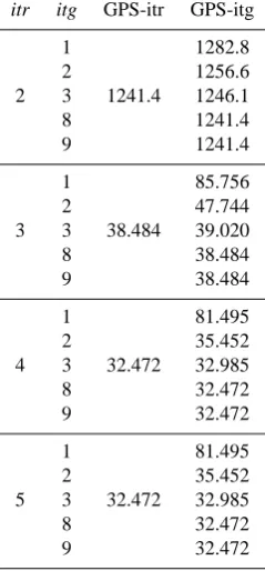
Table 1. Mean value of position-accuracy results (in meter) by GPS
with exact LS method and CORDIC-based approximate rotations.
itr itg GPS-itr GPS-itg
2 1
1241.4
1282.8 2 1256.6 3 1246.1 8 1241.4 9 1241.4
3 1
38.484
85.756 2 47.744 3 39.020 8 38.484 9 38.484
4 1
32.472
81.495 2 35.452 3 32.985 8 32.472 9 32.472
5 1
32.472
81.495 2 35.452 3 32.985 8 32.472 9 32.472
(φij=arctan(aij/ajj)) to the matrix such that the matrix en-tries below the diagonal of A are annihilated, i.e. generate aij0 =0 for
(i,j )= {(2,1)(3,1)...(m,1)(3,2)...(m,2) (11) ...(n+1,n)...(m,n)}.
The resulting matrix is upper triangular and denoted by R. The product of all required Givens rotations forms the or-thogonal matrix QT =
n
Q
j=1
m
Q
i=j+1
G(φij)such that
minwkAw−bk2=minwkRw−QTbk2 (12)
and the solution w can be computed by back substitution. One iteration of the iterative version of the QRD works ex-actly like the QRD but instead of using exact rotations G(φij) that annihilateaij(aij0 =0) CORDIC–based approximate ro-tations are used resulting in|aij0 | = |d||aij|with 0≤ |d|<1. The CORDIC–based approximate Givens rotations are com-puted by determining the shift value`,`∈ {0,1,2,...,b}(b wordlength) corresponding to the CORDIC angle φij(`)= arctan2−`which is closest to the exact rotation angleφij. In-stead of annihilating the matrix elements during the course of the QRD an approximate rotation will only reduce the ma-trix elements by the maximal factor possible withitg spe-cific CORDIC anglesφij(`). This CORDIC–based approxi-mate rotation is applied to the QRD for solving LS problems.
Since the matrix elements below the diagonal are no longer annihilated the QRD procedure using CORDIC–based ap-proximate rotations must iteratively be applied until the ma-trix is ultimately upper triangular. One obtains iterative ver-sions of the QRD distinguished by itg, which determines the accuracy of the approximation of the rotations.
Defining the lower diagonal quantity for iteration itg:
S(itg)= n
X
j=1
m
X
i=j+1
aij(itg)2 (13)
the above algorithm guarantees lim
itg→∞S
(itg)→0
which is equivalent to lim
itg→∞A
(itg)→R and lim itg→∞Q
T (itg)→QT
When we apply this method to the LS problems, which must be solved for positioning in Eq. (8), very few steps, i.e. itgb, of the CORDIC-based approximate rotation are suf-ficient to obtain similar results as using exact rotations. This yields a significant reduction in computational complexity by itg/b(we will show in the following section for real GPS data that even itg=1 gives reasonable results). Furthermore, this method only requiring shift and add operations is very well suited for hardware implementation.
4 Experimental results
4.1 GPS raw data collection
For GPS positioning, a SiGe GN3S Sampler v2 is used to capture the raw GPS data, which are low level signal data (raw intermediate frequency samples) being delivered by the GPS satellite network and processed by the SiGe radio front end (GN3S, 2009). Each GPS satellite continuously broad-casts a navigation message at a rate of 50 bits per second.
The obtained raw GPS data at each measurement point in-cludes information ofm=7 satellites with matched pseudor-anges. 78 raw GPS data records are gained. Afterwards posi-tion calculaposi-tion is done for GPS method for various numbers of required iterations itr (see Sect. 2) and various approxima-tion accuracies itg (see Sect. 3).
4.2 Experimental results
−300 −200 −100 0 100 200 −20
−10 0 10 20 30 40 50
GPS Positioning with real data
exact position mean Position GPS: LS Position GPS: LS mean Position GPS: itg=1 Position GPS: itg=1 mean Position GPS: itg=3 Position GPS: itg=3
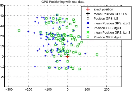
Fig. 3. Positioning results with GPS method.
in Table 1 is the approximation accuracy in QRD. Figures 3 and 4 show the position estimates of GPS positioning. In Table 1 the 3rd column GPS-itr is the accuracy of GPS posi-tioning with exact LS method and the 4th column GPS-itg is the accuracy of GPS positioning using QRD with CORDIC-based approximate rotations for solving LS problems. The results show that with the increasing number of iterations in QRD, the accuracy of GPS-itg also increases. If itg≥8, the accuracy of the exact LS method is achieved. Especially, if itr is big enough, e.g. itr≥3, only one iteration in QRD itg=1 is required to compute the position with reasonable positioning accuracy, which means very coarse approxima-tions are sufficient.
The position estimates of 78 measurements are shown in Fig. 3. GPS position with exact LS (black circles), its mean value (black cross), GPS position using iterative QRD with itg=1 (blue stars), its mean value (blue cross), GPS position using iterative QRD with itg=3 (green squares), its mean value (green cross) and the exact position (red cross) are shown in the figure. All the position results are considered as accuracy of position, i.e. the position estimates subtracted by the exact position (so the exact position is set to(0,0)).
Figure 4 is an enlarged part of Fig. 3. It is obvious to notice that GPS position using QRD with itg=3 (the green squares) are more closer to GPS position with exact LS (black circles) than GPS position using QRD with itg=1 (blue stars). If the number of iterations in QRD increases, i.e.itgincreases, the position results will become more and more similar to the results of exact LS. The mean value of itg=3 is almost the same as the mean value of exact LS (green cross is almost at the same position as black cross in Fig. 4).
5 Conclusion
An iterative LS approach and an iterative version of the QRD using CORDIC-based approximate rotation are applied to position computation. The accuracy of the positioning
re-−150 −100 −50 0 50 100
−15 −10 −5 0 5 10 15 20
GPS Positioning with real data
exact position mean Position GPS: LS Position GPS: LS mean Position GPS: itg=1 Position GPS: itg=1 mean Position GPS: itg=3 Position GPS: itg=3
Fig. 4. Enlarged positioning results with GPS method.
sults of GPS method is compared for various numbers of re-quired iterations itr and various approximation accuracies itg of CORDIC-based approximate rotations by using real GPS data. It is shown that a significant reduction concerning com-putational complexity and hardware requirements can be ob-tained. Furthermore, this method only requiring shift and add operations is very well suited for hardware implementation.
The presented method is very efficient for the implemen-tation of the standard triangulation method based on non-linear LS. In future work we apply this idea to recursive com-putations of the position estimates using Orthogonal DGPS (Chang and Paige, 2003) and Kalman Filter based recursive GPS algorithms (Grewall et al., 2001). In the first case no it-erative LS method is required for positioning which leads to further reduction of the computational effort and the power consumption. In the second case using the square root ver-sion of the Kalman filter (Merwe and Wan, 2001) QRD can be applied and the required approximation accuracy (number of itg) can be investigated to obtain desired position accuracy.
References
Borre, K., Akos, D., Bertelsen, N., Rinder, P., and Jensen, S.: A Software Defined GPS and Galileo Receiver, Birkh¨auser, 2007. Chan, Y. and Ho, K.: A Simple and Efficient Estimator for
Hy-perbolic Location, Signal Processing, IEEE Transactions, 42(8), 1905–1915, 1994.
Chang, X. and Paige, C.: An Orthogonal Transformation Algorithm for GPS Positioning, Society for Industrial and Applied Mathe-matics, 24(5), 1710–1732, 2003.
Djuknic, G. M. and Richton, R. E.: Geolocation and Assisted GPS, IEEE Computer Society, 34(2), 123–125, 2002.
Drane, C., Macnaughtan, M., and Scott, C.: Positioning GSM tele-phones, IEEE Communications Magazine,, 36(4), 46–54, 1998. GN3S Sampler: http://www.sparkfun.com/commerce/product info.
php?products id=8238, 2009.
G¨otze, J.: Iterative Version of the QRD for Adaptive RLS Filtering, SPIE Conference on “Advanced Signal Processing: Algorithms, Architectures and Implementations”, 438–450, 1994.
Grewal, M., Weill, L., and Andrews, A.: Global Positioning Sys-tems, Inertial Navigation and Integration, Wiley & Sons, ISBN-13, 978-0471350323, 2001.
He, Y. and Bilgic, A.: Integrating Location Based Services in Vehicle-to-IMS, Fachgespraech der GI-Fachgruppe KuVS: Application and Services of Location Based Services, Bonn, September 2009.
He, Y., Hueske, K., Gotze, J., and Coersmeier, E.: Efficient Compu-tation of Joint Direction-Of-Arrival and Frequency Estimation, Signal Processing and Information Technology, IEEE Interna-tional Symposium, 144–149, 16–19 December 2008.
Merwe, R. and Wan, E.: The square-root unscented Kalman filter for state and parameter estimation, in: Proc. Int. Conf. Acous. Speech, Signal Process. (ICASSP), 6, 3461–3464, May 2001. Monsmondo, M., Kapov, L., and Kovacic, M.: Bringing
Loca-tion Based Services to IP Multimedia Subsystem, IEEE Melecon 2006, 16–19 May, 746–749, 2006.
Perusco, L. and Michael, K.: Control, Trust, Privacy, and Security: Evaluating Location-Based Services, IEEE Technology and so-ciety magazine, 26(1), 4–16, 2007.
Schiller, J. and Voisard, A.: Location-Bases Services, Morgan Kaufmann by Elservier, ISBN: 1-55860-929-6, 2004.