Information Technology and Control 2019/2/48 278
Model Checking Based Approach
for Compliance Checking
ITC 2/48
Journal of Information Technology and Control
Vol. 48 / No. 2 / 2019 pp. 278-298
DOI 10.5755/j01.itc.48.2.21724
Model Checking Based Approach for Compliance Checking
Received 2018/09/27 Accepted after revision 2019/05/11
http://dx.doi.org/10.5755/j01.itc.48.2.21724
Corresponding author: [email protected]
Fabio Martinelli
Istituto di Informatica e Telematica, Consiglio Nazionale delle Ricerche, Pisa, Italy, e-mail: [email protected]
Francesco Mercaldo
Istituto di Informatica e Telematica, Consiglio Nazionale delle Ricerche, Pisa, Italy Department of Bioscience and Territory, University of Molise, Pesche (IS), Italy, e-mail: [email protected],
Vittoria Nardone
Department of Engineering, University of Sannio, Benevento, Italy, e-mail: [email protected]
Albina Orlando
Istituto per le Applicazioni del Calcolo “M. Picone”, Consiglio Nazionale delle Ricerche, Napoli, Italy, e-mail: [email protected]
Antonella Santone
Department of Bioscience and Territory, University of Molise, Pesche (IS), Italy, e-mail: [email protected]
Gigliola Vaglini
Department of Information Engineering, University of Pisa, Pisa, Italy, e-mail: [email protected]
279 Information Technology and Control 2019/2/48
and complex. In order to solve this problem, another custom-made approach is shown, which accomplishes a pre-processing on the traces to obtain abstract traces, where abstraction is based on the set of temporal logic formulae specifying the system properties. Then, from the set of abstracted traces, we discover a system de-scribed in Lotos, a process algebra specification language; in this way we do not build an operational model for the system, but we produce only a language description from which a model checking environment will auto-matically obtain the reduced corresponding transition system. Real systems have been used as case studies to evaluate the proposed methodologies.
KEYWORDS: Model discovery; process mining; model checking; compliance checking.
1. Introduction
The general idea of process mining techniques is to discover real processes by extracting knowledge from event logs readily available in information systems. These techniques assume that it is possible to re-cord events. Each event e has a set of properties, i.e., resource information (e was executed by John), ac-tivity (e corresponds to a particular procedure), and various data elements. Events are ordered (i.e., no ex-plicit time-stamp is needed) and each event belongs to a particular class (i.e., an activity name). An event refers to a process instance and each process instance is described by a sequence of events referred to as a trace. If we consider activity names, then the trace corresponds to a sequence of such names. An event log is a multi-set of traces, i.e., a collection of traces where some traces may appear multiple times. Process mining has some disadvantages. One of them is that discovered models tend to be large and com-plex, especially on flexible scenarios where process execution involves multiple alternatives. In fact, try-ing to consider every possible process behavior, we can obtain highly complex and incomprehensible models; two typical categories of complex process models are called “lasagna” and “spaghetti” processes because of their intertwined appearance. The reduc-tion of complexity is a major challenge and subject to recent research; abstraction techniques can be useful-ly employed to obtain simpler processes. Other prob-lems are caused by the (essentially, the high quantity of) additional constraints that have to be imposed on the system to guarantee the needed properties. How such constraints can be included in the model may be very hard to be defined. Compliance checking [25] is an important part of the process mining methodolo-gy and it is a relatively novel field of research in that context. Compliance refers to the adherence of the discovered process to internal or external rules and
then deals with verification issues. External rules primarily include laws and regulations but can also reflect industry standards or other external require-ments. Internal rules include management directives, policies and standards. Moreover, compliance check-ing is a strong requirement in the context of internal or external audits.
In the light of the above, our aim is to verify compli-ance through the model checking technique. Accord-ing to process minAccord-ing technique, our idea is to build the formal model of system starting from its exe-cution traces. In particular, we have developed two different kinds of approaches: the first one reusing existing tools, named integrated-tool approach, and the second one, called custom-made approach, aims to discover a process using process algebra language. This custom-made approach aims to fix the main lim-itation of the integrated-tool approach.
More precisely, first we propose the integrated-tool approach using existing tools as ProM1 (a framework
that support a variety of process mining techniques) and CADP [10, 4, 27] (a formal verification environ-ment). In this case, the execution traces from a soft-ware system are extracted. Then, using the “Mine Transition System” plugin in ProM, we obtain a la-belled transition system, that can be easily used to verify formal properties through CADP, as shown in [19]. However, we demonstrated that this choice pres-ents the well-known “state explosion” problem: the models discovered through classical process mining techniques are large and complex.
In order to solve this problem, another custom-made approach has been proposed, where instead of using ProM, we have defined an algorithm producing
Information Technology and Control 2019/2/48 280
stracted model from execution traces. Compliance checking is performed through the model checking of the logic formulae representing the internal or exter-nal rules imposed to the system on its model discov-ered in the form of an abstract Lotos process.
More precisely, we consider that the log refers to the behavior of a distributed system and we can process it to produce distinct traces, each one regarding the be-havior of one device in the system (they have the same resource information); moreover sub-traces repre-senting simple loops (we suppose the use of known methods, for example the α+-algorithm [9]) can be in-dividuated. The description of the possible synchro-nization points, taken from the event properties (i.e., the activity) are used to express the communication among devices. To represent constraints that express particular system requirements, we can use the same formalism and define new traces, not included in the log, but containing existing names connected to activ-ities of the devices. Finally, to address the problem of coping with the high complexity of models obtained by means of automatic process mining, we accom-plish a further pre-processing on the traces to obtain abstract traces. Abstraction is seen as an effective ap-proach to represent readable models, showing aggre-gated activities and hiding irrelevant details.
In our custom-made approach, abstraction is based on the set of temporal logic formulae specifying the system properties. These formulae can be seen also as the declarative representation of the internal and external rules different from the operational ones giv-en by the traces represgiv-enting the system constraints. From the set of abstracted traces, we discover a sys-tem described in Lotos [10], a process algebra speci-fication language; in this way we do not build an op-erational model for the system, like as a Petri net or a transition system, but we produce only a language description from which the model checking environ-ment will automatically obtain the corresponding transition system. Finally, compliance is established through the model checking of the formulae express-ing the compliance rules on the discovered system: any discovered process satisfying the formulae is compliant with the given rules. In this way, we can use existing very efficient model checking environments to establish the compliance of the discovered process without introducing additional concepts or ad hoc model checkers.
A very preliminary work has been presented as poster at ICSOFT 2016 [28].
The remainder of this paper is organized as follows. Section 2 presents a short description of the theoreti-cal background of the work; Section 3 depicts an inte-grated-tool approach able to construct formal models starting from execution traces of a program. Section 4 improves the integrated-tool approach introducing and describing a custom-made approach able to build reduced formal models, also a simple working exam-ple is presented. Moreover, the section illustrates the technique for model discovery and gives the results of the model checking of some properties. Section 5 shows the experimental results achieved during the evaluation of the custom-made approach. Section 6 elicits the limitations of our approach. Section 7 dis-cusses some related work and Section 8 presents the conclusions.
2. Background
Some basic concepts of process algebra specifications and model checking of temporal logic formulae are re-called in this section.
2.1. Basic Lotos
Let us now recall the main concepts of Basic Lotos [10], which is widely used in the specification of con-current and distributed systems. A Basic Lotos pro-gram is defined as:
process ProcName := P where Env
endproc,
where P is a process, process ProcName := P is a pro-cess declaration and is a Env propro-cess environment, i.e., a set of process declarations. A process is the com-position, by means of a set of operators, of a finite set E = {i, a, b,...} of atomic events (or actions). Each oc-currence of an action in E represents an event of the system. An occurrence of an event a ∈ E – {i} rep-resents a communication on the gate a. Event i does not correspond to a communication and it is called
the unobservable event. The operational semantics
281 Information Technology and Control 2019/2/48
as S(P), i.e., an automaton whose states correspond
to processes (the initial state corresponds to P) and whose transitions (arcs) are labeled by events in E. Reader unfamiliar with Lotos process syntax can re-fer to [11].
2.2. Model Checking Selective Mu-Calculus Formulae
In the model checking framework [6], systems are modelled as transition systems and requirements are expressed as formulae in a temporal logic. Model checkers accept two inputs, a transition system and a temporal formula, and return “true” if the system sat-isfies the formula and “false” otherwise. We consider formulae expressed in the selective mu-calculus tem-poral logic [2]. The basic characteristic of the selective mu-calculus is that the actions relevant for checking a formula are those ones explicitly mentioned in the modal operators used in the formula itself.
(1) The syntax of the selective mu-calculus is the fol-lowing: where K, R are sets of events in Ε, while Z ranges over a set of variable names; μZ.ϕ is the least fix-point of the recursive equation Z=ϕ, while νZ.ϕ is the greatest one.
The selective modal operators 〈K〉Rϕ and [K]Rϕ substi-tute the standard modal operators 〈K〉ϕ and [K]ϕ:
_ [K]Rϕ is satisfied by a state which, for every
performance of a sequence of actions not belonging
to R∪K, followed by an action inK, evolves to a state
obeying ϕ.
_ 〈K〉Rϕ is satisfied by a state which can evolve to a
state obeying ϕ by performing a sequence of actions not belonging to R∪K, followed by an action in K. A transition system T satisfies a formula ϕ, written
T⊨ϕ, if and only if p⊨ϕ, where p is the initial state of
T. Moreover, a process P satisfies ϕ if S(P) satisfies ϕ. The precise and formal definition of satisfaction of selective mu-calculus formulae can be found in [2]. The basic characteristic of the selective mu-calculus is that the actions relevant for checking a formula ϕ are those ones explicitly mentioned in the modal op-erators used in the formula itself. Thus we define the
set O(ϕ) of occurring actions of a formula ϕ as the
union of all sets K and R appearing in the modal oper-ators ([K]Rψ, 〈K〉Rψ) occurring in ϕ. A ρ - bisimulation can be defined, formally characterizing the notion of “the same behavior with respect to a set ρ of actions”:
two transition systems are ρ -equivalent if a ρ -
bisi-mulation relating their initial states exists.
The definition of ρ -bisimulation is based on the concept of α - ending path: an α - ending path is a sequence of transitions, labelled by events not in ρ, and followed by a transition labelled by the event α in ρ. Two states S1 and S2 are ρ - bisimilar if and only
if for each α -ending path starting from S1 and
end-ing into S1', there exists an α - ending path starting
from S2 and ending into a state ρ - bisimilar to S1', and
vice-versa. If a ρ -bisimulation relating the initial states of two transition systems exists, then the two systems are ρ - equivalent. As conclusion, in [2] the following theorem is proved:
Theorem 1. Two transition systems are ρ - equivalent if and only if they satisfy the same set of formulae with occurring events in ρ.
The interesting consequence of the theorem is that a formula of the selective mu-calculus with occurring events in a set ρ can be checked on any transition sys-tem ρ - equivalent to the standard one, in particular on the system with the lowest number of states.
3. Integrated-Tool Approach
In order to link model checking verification closer to real implementation allowing to perform compliance checking an approach integrating existing tools has been proposed in this section.
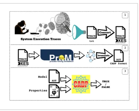
Figure 1 shows the work-flow of the integrated-tool approach able to model and verify a system starting from its execution traces. It is mainly based on three steps:
_ First step(see Figure 1 (1)): It starts from the
Information Technology and Control 2019/2/48 282
on objects. Starting from this textual format traces an eXtensible Event Stream format (XES) is generated. XES is an IEEE XML-based standard for event logs. During this conversion process the traces are filtered removing all the unnecessary information.
_ Second step (see Figure 1 (2)): It creates the
model from the XES traces using Process Mining Workbench (ProM)2. ProM is an extensible
framework that supports a wide variety of process mining techniques in the form of plug-ins. It is an independent platform as it is implemented in Java, and can be downloaded free of charge. From the XES Event Log, using the “Mine Transition System” plugin in ProM developed by H.M.W. Verbeek, a labelled transition system is obtained. The transitions correspond to the events in the log, whereas a state corresponds to a situation in between two events.
_ Third step (see Figure 1 (3)): It applies the
model checking technique. Once the formal model has been retrieved, it is easily used to verify properties using a model checker tool. This step checks the sets of logic properties against the formal model obtained starting from the feature set, as described above. In our approach, the Construction and Analysis of Distributed Processes (CADP) tool [10] is invoked as formal
2 http://www.promtools.org/ Figure 1
The work-flow of the integrated approach
two transition systems are
𝜌𝜌𝜌𝜌
-
equivalent
if a
𝜌𝜌𝜌𝜌
-
bisimulation relating their initial states exists.
The definition of
𝜌𝜌𝜌𝜌
-bisimulation is based on the concept of
𝛼𝛼𝛼𝛼
-ending path: an
𝛼𝛼𝛼𝛼
-ending
path is a sequence of transitions, labelled by events not in
𝜌𝜌𝜌𝜌
, and followed by a transition labelled by the
event
𝛼𝛼𝛼𝛼
in
𝜌𝜌𝜌𝜌
. Two states
𝑆𝑆𝑆𝑆
1and
𝑆𝑆𝑆𝑆
2are
𝜌𝜌𝜌𝜌
-bisimilar if and only if for each
𝛼𝛼𝛼𝛼
-ending path starting
from
𝑆𝑆𝑆𝑆
1and ending into
𝑆𝑆𝑆𝑆
1′, there exists an
𝛼𝛼𝛼𝛼
-ending path starting from
𝑆𝑆𝑆𝑆
2and ending into a state
𝜌𝜌𝜌𝜌
-bisimilar to
𝑆𝑆𝑆𝑆
1′, and vice-versa. If a
𝜌𝜌𝜌𝜌
-bisimulation relating the initial states of two transition systems
exists, then the two systems are
𝜌𝜌𝜌𝜌
-
equivalent
. As conclusion, in [2] the following theorem is proved:
Theorem 1.
Two transition systems are
𝜌𝜌𝜌𝜌
-equivalent if and only if they satisfy the same set of
formulae with occurring events in
𝜌𝜌𝜌𝜌
.
The interesting consequence of the theorem is that a formula of the selective mu-calculus with
occurring events in a set
𝜌𝜌𝜌𝜌
can be checked on any transition system
𝜌𝜌𝜌𝜌
-equivalent to the standard one,
in particular on the system with the lowest number of states.
3 Integrated-Tool Approach
In order to link model checking verification closer to real implementation allowing to perform
compliance checking an approach integrating existing tools has been proposed in this section.
Figure 1. The work-flow of the integrated approach
Figure 1 shows the work-flow of the integrated-tool approach able to model and verify a system
starting from its execution traces. It is mainly based on three steps:
•
First step (see Figure 1 (1)):
It starts from the execution traces of a program obtained from the
execution of a software system. Traces are usually stored in text files and they contain both
static and dynamic information retrieved during software execution. Static information regards,
for instance, class structure in terms of methods and fields. Dynamic information refers to
method calls, field access in read or write mode and synchronization on objects. Starting from
this textual format traces an eXtensible Event Stream format (XES) is generated. XES is an
IEEE XML-based standard for event logs. During this conversion process the traces are filtered
removing all the unnecessary information.
•
Second step (see Figure 1 (2)):
It creates the model from the XES traces using Process Mining
verification environment. In order to apply CADP, the transition system obtained is converted into the input format of CADP, parsing the automaton ProM file. Moreover, the property, written in selective mu-calculus, can be equivalently transformed in the syntax of the logic used by the CADP environment.
3.1. Result Using the Integrated-Tool Approach
In order to evaluate the integrated-tool approach, an example of a real system obtained from the ProM website3 has been considered. It describes a
realis-tic transaction process within a banking context. In the integrated-tool approach evaluation, the first step has been skipped because the considered real case study has already developed and made available from the repository of the ProM database. The ana-lysed process contains all sort of monetary checks, authority notifications, and logging mechanisms responding to the new degree of responsibility and accountability that current economic environments demand. As stated in [22], “the banking regulation states that serial numbers must be compared with an external database governed by a recognized inter-national authority (“Check Authority Serial Num-bers CASN”). In addition, the bank of the case study decided to incorporate two complementary checks to its policy: an internal bank check (“Check Bank Serial Numbers CBSN”), and a check among the da-tabases of the bank consortium this bank belongs to (“Check Inter-Bank Serial Numbers CIBSN”). At a given point, due to technical reasons (i.e., peak hour network congestion, malfunction of the soft-ware, deliberated blocking attack, etc.), the external check CASN is no longer performed, contradicting the modeled process, i.e., all the running instances of the process involving cash payment can proceed without the required check”.
According with our preliminary approach, we formu-late the above anomaly in mu-calculus logic formulae using the following pattern:
The formula φ means that for each action a not pre-ceded by b and c and for each action b not prepre-ceded by c, eventually the action c will be performed.
283 Information Technology and Control 2019/2/48
The formula φ expresses the above anomalous situ-ation that the external check CASN is no longer per-formed.
involving cash payment can proceed without the required check”.
According with our preliminary approach, we formulate the above anomaly in mu-calculus logic formulae using the following pattern:
The formula means that for each action a not preceded by b and c and for each action b not preceded by c, eventually the action c will be performed.
The formula expresses the above anomalous situation that the external check CASN is no longer performed.
.
(2)
The model checker returns “false” when evaluating , stating that the anomalous situation is immediately detected, identifying the anomalous subprocess (process cash payment), and eventually taking the necessary countermeasures. The advantage is that it is better to discover the error as soon as possible. It is worth noting that when a property does not hold, the model checking algorithm generates a counter-example, i.e., an execution trace leading to a state in which the property is violated. This ability to generate counter-examples, which can be exploited to pinpoint the cause of an error, is the main advantage of model checking, as compared to other well-known techniques for software verification, as abstract interpretation-based static analysis.
In the used dataset there are six different scenarios: (i) 2000-all-noise; (ii) 2000-all-nonoise; (iii) 2000-scen1; (iv) 2000-scen2; (v) 10000-all-noise; and (vi) 10000-all-nonoise.
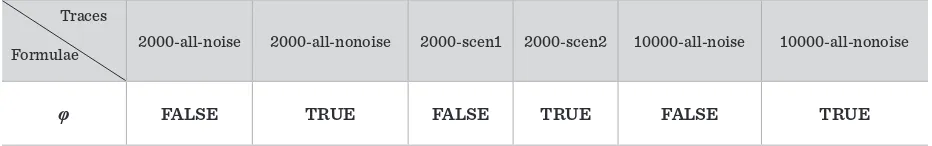
Table 1. Property Results
Traces
Formulae
2000-all-noise2000-all-nonoise2000-scen12000-scen210000-all-noise10000-all-nonoise
𝜑𝜑 FALSE TRUE FALSE TRUE FALSE TRUE
1[CASN]{CIBSN,CBSN}[CIBSN]{CBSN}1
1(
X. Att[CBSN]AX)2[CASN]{CIBSN,CBSN}[CBSN]{CIBSN}2
2(
X. Att[CIBSN]AX)3[CIBSN]{CASN,CBSN}[CASN]{CBSN}3
3(
X. Att[CBSN]AX)4[CIBSN]{CASN,CBSN}[CBSN]{CASN}4
4(
X. Att[CASN]AX)5[CBSN]{CASN,CIBSN}[CASN]{CIBSN}5
5(
X. Att[CIBSN]AX)6[CBSN]{CASN,CIBSN}[CIBSN]{CASN}6
6(
X. Att[CASN]AX)
1
2
3
4
5
6
(2)
The model checker returns “false” when evaluating φ, stating that the anomalous situation is immedi-ately detected, identifying the anomalous subprocess (process cash payment), and eventually taking the necessary countermeasures. The advantage is that it is better to discover the error as soon as possible. It is worth noting that when a property does not hold, the model checking algorithm generates a count-er-example, i.e., an execution trace leading to a state in which the property is violated. This ability to gen-erate counter-examples, which can be exploited to pinpoint the cause of an error, is the main advantage of model checking, as compared to other well-known
techniques for software verification, as abstract in-terpretation-based static analysis.
In the used dataset there are six different scenarios: (i) all-noise; (ii) all-nonoise; (iii) 2000-scen1; (iv) 2000-scen2; (v) 10000-all-noise; and (vi) 10000-all-nonoise.
The first item of the string is the number of traces in the XES event stream file. “noise” (resp. “nonoise”) specifies if the considered traces are (resp. are not) affected by the noise. Furthermore, there are two files used in [22] which present two possible scenar-ios: Serial Number Check and Receiver Preliminary Profiling, i.e., “scen1” and “scen2”, respectively. The results of the verification of φ formula are: “True” in 2000-all-nonoise, 2000-scen2 and 1000-all-nonoise, “False” in the other cases.
Table 1 shows the results achieved by φ formula. As pointed out from the results, φ is false in some scenar-ios stating that anomalous traces occur. In particular, anomalous situations are detected in the presence of noise which could be due for different reasons, i.e., de-liberate blocking attack, peak hour network conges-tion or malfuncconges-tion of the software.
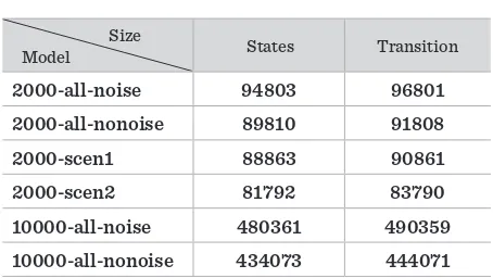
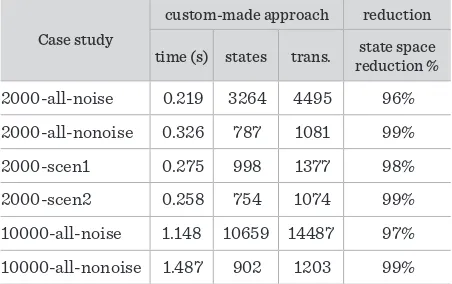
The sizes of models used in the experimental evalu-ation are shown in Table 2. The size of a model is ex-pressed in terms of states and transitions. As shown in Table 2 the number of states and transitions grows dramatically according to the growing of number of traces. As a simple example the reader can refer the last two rows of Table 2. This means that our pre-liminary approach suffers of the well-known states explosion problem. To fix this weakness we propose another solution able to directly build a reduced mod-el starting from the execution traces. This modmod-el is presented in Section 4.
Table 1
φ Property results
Traces
Formulae 2000-all-noise 2000-all-nonoise 2000-scen1 2000-scen2 10000-all-noise 10000-all-nonoise
Information Technology and Control 2019/2/48 284
In order to better analyze the results obtained by the φ formula, we defined additional eight formulae able to check every single trace belonging to a specific sce-nario. In particular, these formulae investigate the cause of φ failure. The specified properties are ex-pressed by the following selective mu-calculus:
The first item of the string is the number of traces in the XES event stream file. “noise” (resp. “nonoise”) specifies if the considered traces are (resp. are not) affected by the noise. Furthermore, there are two files used in [22] which present two possible scenarios: Serial Number Check and Receiver Preliminary Profiling, i.e., “scen1” and “scen2”, respectively. The results of the verification of formula are: “True” in 2000-all-nonoise, 2000-scen2 and 1000-all-nonoise, “False” in the other cases. Table 1 shows the results achieved by formula. As pointed out from the results, is false in some scenarios stating that anomalous traces occur. In particular, anomalous situations are detected in the presence of noise which could be due for different reasons, i.e., deliberate blocking attack, peak hour network congestion or malfunction of the software.
The sizes of models used in the experimental evaluation are shown in Table 2. The size of a model is expressed in terms of states and transitions. As shown in Table 2 the number of states and transitions grows dramatically according to the growing of number of traces. As a simple example the reader can refer the last two rows of Table 2. This means that our preliminary approach suffers of the well-known states explosion problem. To fix this weakness we propose another solution able to directly build a reduced model starting from the execution traces. This model is presented in Section 4.
Table 2. Model Size
Size
Model States Transition 2000-all-noise 94803 96801 2000-all-nonoise 89810 91808 2000-scen1 88863 90861 2000-scen2 81792 83790 10000-all-noise 480361 490359 10000-all-nonoise 434073 444071
In order to better analyze the results obtained by the formula, we defined additional eight formulae able to check every single trace belonging to a specific scenario. In particular, these formulae investigate the cause of failure. The specified properties are expressed by the following selective mu-calculus:
(3)
1 CASN tt CIBSN tt CBSN tt
2CASNff CIBSN ff CBSN ff
3 CIBSN tt CBSN ttCASN ff
4 CASN tt CBSN ttCIBSNff
5 CASN tt CIBSN ttCBSN ff
6 CASN ttCIBSNffCBSN ff
7 CIBSN ttCASNffCBSNff
8 CBSN ttCASNffCIBSNff
(3) Table 2
φ Model and size
Size
Model States Transition
2000-all-noise 94803 96801
2000-all-nonoise 89810 91808
2000-scen1 88863 90861
2000-scen2 81792 83790
10000-all-noise 480361 490359
10000-all-nonoise 434073 444071
Roughly speaking, the formulae have the following meaning:
_ φ1 checks if all the three actions (CASN, CIBSN and
CBSN) are performed.
_ φ2 checks if all CASN, CIBSN and CBSN are not
performed.
_ φ3 checks if CIBSN and CBSN actions are
performed and the CASN action is not performed. _ φ4 checks if CASN and CBSN actions are performed
and the CIBSN action is not performed.
_ φ5 checks if CIBSN and CASN actions are
performed and the CBSN action is not performed. _ φ6 checks if CIBSN and CBSN actions are not
performed and the CASN action is performed. _ φ7 checks if CBSN and CASN actions are not
performed and the CIBSN action is performed. _ φ8 checks if CIBSN and CASN actions are not
performed and the CBSN action is performed. Table 3 shows the results obtained during the verifica-tion of the formulae specified above. In particular, Ta-ble 3 is organized as follow: the above specified formu-lae are described in the rows, while the scenarios in the columns. Each single model represents a single realis-tic banking transaction trace. The first four sets have 2000 different traces, so 2000 formal models. The last two have 10000 traces corresponding to 10000 differ-ent formal models. The last row is the total number of the analyzed traces resulting true to the formulae. This value is obtained by adding to each other the values in the corresponding column. The table shows the
num-Table 3
Detailed properties
Formulae Traces
all-noise all-nonoise scen1 scen2 all-noise all-nonoise
φ1 531 708 327 701 2478 3326
φ2 1293 1292 1348 1299 6678 6674
φ3 67 0 325 0 249 0
φ4 50 0 0 0 259 0
φ5 49 0 0 0 260 0
φ6 5 0 0 0 28 0
φ7 3 0 0 0 18 0
φ8 2 0 0 0 30 0
285 Information Technology and Control 2019/2/48
ber of true achieved by every type of analyzed model. As the results shown and according to the “True” val-ues of the φ formula, the files with no noise and the files of second scenario have all the traces of transactions correct, i.e., whenever a client executed a payment in cash, the three required actions have been performed. This result is highlighted by positive values of φ1 and φ2
and the values equal to zero achieved by the other for-mulae. In the “False” cases the anomalous situations are caused by several reasons. In the “scen1” scenario bad and unsafe transactions occur because only the action CASN has not been performed. Finally, in the scenarios affected by noise the causes of failure occur because one or two required actions are not performed during a payment in cash.
4. Custom-Made Approach
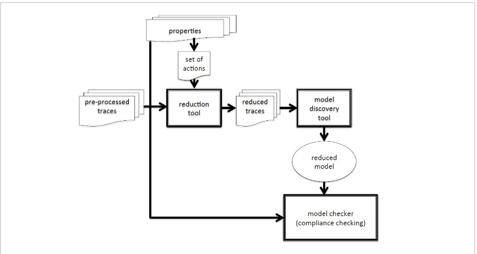
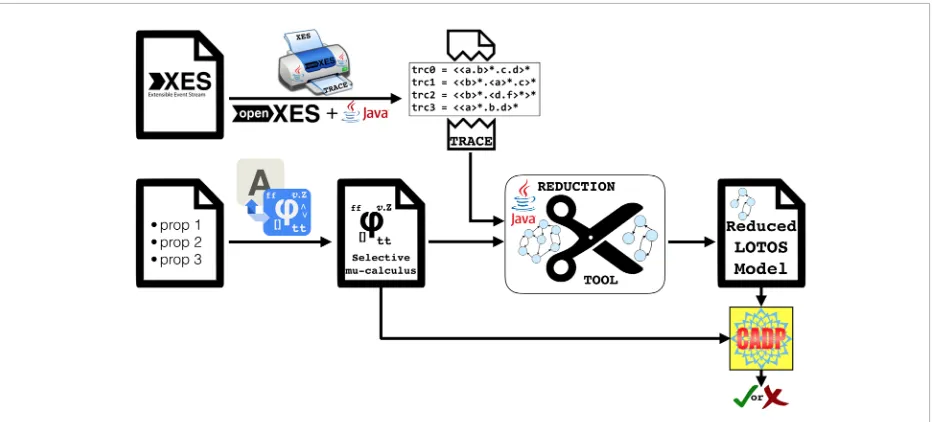
As stated in Section 3 the integrated-tool approach at-tempt suffers of the state explosion problem. In order to address this limitation we have developed another approach able to fix the state explosion problem. The basic steps of the new methodology that we are going to propose are summarized in Figure 2. In this
section, we assume that the log is pre-processed so that the traces are rearranged to obtain separate trac-es for each device in a distributed system exploiting the source of each activity. Further, we give each ac-tivity a different name; moreover simple loops are solved using α+-algorithm; after this pre-processing, we consider that it is now possible to describe the traces derived from the log by means of the simple language defined in the next subsection. Successively, names corresponding to activities performing equal communication among devices are given a new equal name and, finally, system constraints may be included in the specification by means of new traces. Proper-ty-driven reductions can be performed on the result-ing traces to obtain an abstract model of the system in the process algebra Lotos. This model will be model checked against the required properties to verify its compliance.
4.1. Trace-Based System Specification
A specification as we will use in the following can be derived from the log of a physical system or from the instrumentation of a software system. The lan-guage we assume be used to define the traces obtained through the log pre-processing is the following.
Figure 2 The methodology
Figure 2. The methodology
4.1 Trace-Based System Specification
A specification as we will use in the following can be derived from the log of a physical system or from the instrumentation of a software system. The language we assume be used to define the traces obtained through the log pre-processing is the following.
Definition 1 (Trace) Let Ε= {𝑒𝑒𝑒𝑒1,𝑒𝑒𝑒𝑒2, … } be a set of activity names, a trace of such names can be built
up by the following syntax:
𝑡𝑡𝑡𝑡 ∷=𝑒𝑒𝑒𝑒|𝑡𝑡𝑡𝑡.𝑡𝑡𝑡𝑡|〈𝑡𝑡𝑡𝑡〉∗|𝜆𝜆𝜆𝜆, (4)
where 𝑒𝑒𝑒𝑒 ∈ Ε and 𝜆𝜆𝜆𝜆 is the empty sequence.
The operator “.” represents trace concatenation: usually it is omitted. The operator “*” represents
the iteration of a trace and it turns out that 〈〈𝑡𝑡𝑡𝑡〉∗〉∗ is equivalent to 〈𝑡𝑡𝑡𝑡〉∗. Moreover, 〈𝜆𝜆𝜆𝜆〉∗ is equivalent to 𝜆𝜆𝜆𝜆. The following definitions are of interest.
Definition 2 (Alphabet, Branching names) Let 𝑇𝑇𝑇𝑇 be a set of traces:
• 𝛼𝛼𝛼𝛼𝑇𝑇𝑇𝑇 is the alphabet of 𝑇𝑇𝑇𝑇, and
• 𝐶𝐶𝐶𝐶𝑒𝑒𝑒𝑒(𝑇𝑇𝑇𝑇) is the set of pairs defined as follows:
𝐶𝐶𝐶𝐶𝑒𝑒𝑒𝑒(𝑇𝑇𝑇𝑇) = {(𝑒𝑒𝑒𝑒,𝑒𝑒𝑒𝑒′)|𝑡𝑡𝑡𝑡1=𝑠𝑠𝑠𝑠.𝑒𝑒𝑒𝑒.𝑡𝑡𝑡𝑡 ∈ 𝑇𝑇𝑇𝑇,𝑡𝑡𝑡𝑡2=𝑠𝑠𝑠𝑠.𝑒𝑒𝑒𝑒′.𝑡𝑡𝑡𝑡′∈ 𝑇𝑇𝑇𝑇,𝑒𝑒𝑒𝑒 ≠ 𝑒𝑒𝑒𝑒′ 𝑎𝑎𝑎𝑎𝑛𝑛𝑛𝑛𝑎𝑎𝑎𝑎 𝑠𝑠𝑠𝑠,𝑡𝑡𝑡𝑡,𝑡𝑡𝑡𝑡′∈ Ε′}
Information Technology and Control 2019/2/48 286
Definition 1 (Trace). Let E = {e1, e2,…} be a set of
activ-ity names, a trace of such names can be built up by the following syntax:
4.1 Trace-Based System Specification
A specification as we will use in the following can be derived from the log of a physical system or from the instrumentation of a software system. The language we assume be used to define the traces obtained through the log pre-processing is the following.
Definition 1 (Trace) Let be a set of activity names, a trace of such names can be built
up by the following syntax:
(4)
where and is the empty sequence.
The operator “.” represents trace concatenation: usually it is omitted. The operator “*”
represents the iteration of a trace and it turns out that is equivalent to . Moreover, is equivalent to . The following definitions are of interest.
Definition 2 (Alphabet, Branching names) Let be a set of traces: • is the alphabet of , and
• is the set of pairs defined as follows:
For example, given ,
• ;
• .
After having obtained from the log the set of traces of activity names, our aim is to obtain from the model of the distributed system as Lotos processes composed in parallel. The first step of our method is:
1. Individuation of the traces of each component of the distributed system in isolation (the layout)
We give the following definition.
Definition 3 (Layout Specification) Given a set of traces of activity names derived from a log, the Layout Specification of a distributed system is , where each has a distinct alphabet
, and each activity in has the same source, different from that of each other .
The second step consists in the representation in the traces of communications performed among devices; the activity definitions in the log allows the individuation of corresponding communication activities. This step is called:
{e1,e2,...}
t::e|t.t| t *|
e
t * * t *
*
T
T T
Be(T)
Be(T){(e,e1) |t
1s.e.ts.e'.t'T,ee' and s,t,t''}
T{a.b.c.d.e, a.b.g.h}
T{a,b,c,d,e,g,h}
Be(T){(c,g)}
T T
LS{T1,...,Tn} Ti
Ti Ti Tj
(4)
where e ∈ E and λ is the empty sequence.
The operator “. ” represents trace concatenation: usu-ally it is omitted. The operator “ ” represents the itera-tion of a trace and it turns out that 〈〈t〉*〉* is equivalent to 〈t〉*. Moreover, 〈λ〉* is equivalent to λ. The following definitions are of interest.
Definition 2 (Alphabet, Branching names). Let T be a
set of traces:
_ αT is the alphabet of T, and
_ Be(T) is the set of pairs defined as follows: 𝐶𝐶𝐶𝐶𝐶𝐶𝐶𝐶(𝑇𝑇𝑇𝑇)={(𝐶𝐶𝐶𝐶,𝐶𝐶𝐶𝐶′)|𝑡𝑡𝑡𝑡
1=𝑠𝑠𝑠𝑠.𝐶𝐶𝐶𝐶.𝑡𝑡𝑡𝑡 ∈ 𝑇𝑇𝑇𝑇,𝑡𝑡𝑡𝑡2=𝑠𝑠𝑠𝑠.𝐶𝐶𝐶𝐶′.𝑡𝑡𝑡𝑡′∈ 𝑇𝑇𝑇𝑇,𝐶𝐶𝐶𝐶 ≠𝐶𝐶𝐶𝐶′𝑎𝑎𝑎𝑎𝑛𝑛𝑛𝑛𝑎𝑎𝑎𝑎𝑠𝑠𝑠𝑠,𝑡𝑡𝑡𝑡,𝑡𝑡𝑡𝑡′∈ Ε′}
𝐶𝐶𝐶𝐶𝐶𝐶𝐶𝐶(𝑇𝑇𝑇𝑇)={(𝐶𝐶𝐶𝐶,𝐶𝐶𝐶𝐶′)|𝑡𝑡𝑡𝑡
1=𝑠𝑠𝑠𝑠.𝐶𝐶𝐶𝐶.𝑡𝑡𝑡𝑡 ∈ 𝑇𝑇𝑇𝑇,𝑡𝑡𝑡𝑡2=𝑠𝑠𝑠𝑠.𝐶𝐶𝐶𝐶′.𝑡𝑡𝑡𝑡′∈ 𝑇𝑇𝑇𝑇,𝐶𝐶𝐶𝐶 ≠𝐶𝐶𝐶𝐶′𝑎𝑎𝑎𝑎𝑛𝑛𝑛𝑛𝑎𝑎𝑎𝑎𝑠𝑠𝑠𝑠,𝑡𝑡𝑡𝑡,𝑡𝑡𝑡𝑡′∈ Ε′}
For example, given T= {a.b.c.d.e, a.b.g.h},
_ αT = {a, b, c, d, e, g, h };
_ Be(T) = {(c, g)}.
After having obtained from the log the set T of trac-es of activity namtrac-es, our aim is to obtain from T the model of the distributed system as Lotos processes composed in parallel. The first step of our method is:
1 Individuation of the traces of each component of
the distributed system in isolation (the layout) We give the following definition.
Definition 3 (Layout Specification). Given a set of traces of activity names derived from a log, the Layout Specification of a distributed system is LS = {T1, …, Tn}, where each Ti has a distinct alphabet αTi, and each activity in Ti has the same source, dif-ferent from that of each other Tj.
The second step consists in the representation in the traces of communications performed among devices; the activity definitions in the log allows the individuation of corresponding communica-tion activities. This step is called:
2 Specification of the synchronization between
components (the flow)
Definition 4 (Flow Specification. Renaming func-tion ⇝). Consider the Layout Specification LS and the set C = {c1, …, cm}, where cj = {cj1, …, cjk}, 1 ≤ j ≤ m, where the names in the same tuple individuate cor-responding communication activities in the log.
The renaming function S is such that ∀j, s∈[1..m], S(cj) = ej, and ej ∉ αLS, moreover, for j ≠ s it is S(cj) ≠S(cs). The Flow Specification is FS = LS⇝S(C), which is the result of the renaming. From now on we will use S(C) for {S(c1), …, S(cm)}.
S renames all elements of C using the same new name for all elements of the same tuple of C; obvi-ously the new name given to each tuple is different from those chosen for the other tuples and from all other names in the traces. Table 5 shows an exam-ple of renaming function.
The third (possibly not present) step consists in the definition of specific requirements for the system. They are expressed as traces that are built using the alphabet of the Flow specification. This step is:
3 Construction of the traces that model
con-straints (the control)
Definition 5 (Control specification). Consider the Flow specification FS, CS = {t1, …, tc} is a unique set of finite traces on αFS (also called control traces) with a unique activity source different from any other in FS. CS is the Control Specification of the system. CS is a set of traces not retrieved from the log; note that, all events in the Control Specifica-tion result in communicaSpecifica-tion events. A wide class of constraints can be expressed by means of such kind of traces, also binding the behavior of several system components. Obviously a Control Specifi-cation expresses system requirements that are due, but that the system does not necessarily respect; actually, imposing such constraints can cause deadlocks in the system. The trace-based System Specification (SS for short) is defined as follows. Definition 6 (System Specification). A System Specification SS can be either a Flow Specification only, SS = (LS ⇝ S(C)), or a Flow Specification plus a Control Specification in the same language, SS = (LS ⇝ S(C))∪CS.
4.2. The Working Example
287 Information Technology and Control 2019/2/48
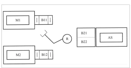
The machine M1 (M2) performs an operation op1 (op2) on a raw part of type t1 (t2). After the operation op1 (op2) is performed, the part is available in the out-put buffering area B11 (B12) and is picked up by the robot R to be moved into the input buffering area B21 (B22) of the assembly station. The finished product must be assembled from two parts of type t1 and one part of type t2; the assembly station must wait for the robot having moved a second part of type t2 in its in-put buffering area after it is set free from the station itself. To guarantee this result, the control may spec-ify that the non-deterministic behavior of the robot (on choice between a part of type t1 and t2, when both are available) must be restricted to always move two parts of type t1 for each part of type t2. This control specification supplies a bit of further information with respect to the abstract requirement on the cor-rect assembling of the finished products: it also con-strains the free behavior of the system to perform a subset of the acceptable computations.
The traces of the components of the working example are very simple and self-explaining and we just report them in Table 4 (machines and buffers are indexed). We have considered buffers of one position only, but the specification can be easily extended.
Table 5 shows the renaming function S which defines the flow of the parts; the events in αLS that are not present in the table are assumed unchanged and rep-resent the internal behavior of each component. The derived Flow Specification, FS, is shown in Table 6. The constraints to be imposed over the system can be expressed by the Control Specification, CS, in Table 6. The trace C1 requires that at least one occurrence of the event part2_load happens after two occurrences of the event part1_mov, whereas C2 requires that at Figure 3
Plant of the system
Figure 3. Plant of the system
Table 4. Layout Specification, LS Machines , with
Buffering areas , with
Robot
Assembly Station 𝐴𝐴𝑆𝑆
The machine M1 (M2) performs an operation op1 (op2) on a raw part of type t1 (t2). After
the operation op1 (op2) is performed, the part is available in the output buffering area 11B ( 12B ) and
is picked up by the robot R to be moved into the input buffering area B21 (B22) of the assembly
station. The finished product must be assembled from two parts of type t1 and one part of type t2; the assembly station must wait for the robot having moved a second part of type t2 in its input buffering area after it is set free from the station itself. To guarantee this result, the control may specify that the non-deterministic behavior of the robot (on choice between a part of type t1 and t2, when both are available) must be restricted to always move two parts of type t1 for each part of type t2. This control specification supplies a bit of further information with respect to the abstract requirement on the correct assembling of the finished products: it also constrains the free behavior of the system to perform a subset of the acceptable computations.
The traces of the components of the working example are very simple and self-explaining and we just report them in Table 4 (machines and buffers are indexed).
We have considered buffers of one position only, but the specification can be easily extended.
Table 5 shows the renaming function which defines the flow of the parts; the events in that are not present in the table are assumed unchanged and represent the internal behavior of each component. The derived Flow Specification, FS, is shown in Table 6.
Mi i[1,2]
Mi{Mi_start.Mi_opMi_end*}
Bij i,j[1,2]
Bij{Bij_in.Bij_out*} R
R{R_init.R_start1R_op.R_end1*,R_init.R_start2.R_op2.R_end2*}
AS{AS_start.AS_load1.AS_load2.AS_op.AS_end*,
AS_start.AS_load1.AS_load2.AS_op.AS_end*}
S
LS
Table 5
Renaming function, S
∀i ∈ [1..n]:
S(Mi_end, B1i_in) = parti_aval
(B1i_out, R_starti) = parti_mov S(R_endi, B2i_in) = parti_load S(B2i_out, AS_loadi) = parti_work
Table 6
Trace-based System Specification, SS
Flow Specification (FS) Machines Mi, withi ∈ [1,2]
Mi= {〈Mi_start.Mi_op.parti_aval〉* }
Machines’ buffering areas B1i, with i ∈ [1,2]
B1i = {〈parti_aval.parti_mov〉* }
Assembly station’s buffering area B2i, with i ∈ [1,2]
B1i = {〈parti_load.parti_work〉*}
Robot R
R {〈R_init.part1_mov.R_op1.part1_load〉*,
〈R_init.part2_mov.R_op2.part2_load〉*}
Assembly Station AS
AS = {〈AS_start.part1_work.part2_work.AS_op.AS_end〉*,
〈AS_start.part2_work.part1_work.AS_op.AS_end〉*}
Control Specification (CS)
C= {〈part1_mov.part1_mov.part2_load〉*,
〈part2_mov.part1_mov.part1_load〉*}
Table 4
Layout Specification, LS
MachinesMi, withi∈ [1,2]
Mi = {〈Mi_start.Mi_op.Mi_end〉*} Buffering areas Bij, with i, j∈[1, 2]
Bij = {〈Bij_in.Bij_out〉*}
RobotR
R = {〈R_init.R_start1.R_op.R_end1〉*, 〈R_init.R_start2.R_op2.R_end2〉*}
Assembly Station AS
AS = {〈AS_start.AS_load1.AS_load2.AS_op.AS_end〉*,