* Corresponding author. Tel.: +234-803-4131860; E-mail address: [email protected] Manuscript History:
Comparative Performance Evaluation of Three Image Compression
Algorithms
Jide Julius Popoola
*and Michael Elijah Adekanye
Department of Electrical and Electronics Engineering, School of Engineering and
Engineering Technology, Federal University of Technology, Akure, Nigeria
Abstract
The advent of computer and internet has brought about massive change to the ways images are being managed. This revolution has resulted in changes in image processing and management as well as the huge space requirement for images’ uploading, downloading, transferring and storing nowadays. In guiding against this huge space requirement, images need to be compressed before either storing or transmitting. Several algorithms or techniques on image compression had been developed in literature. In this study, three of these image compression algorithms were developed using MATLAB codes. The three algorithms developed are discrete cosine transform (DCT), discrete wavelet transform (DWT) and set partitioning in hierarchical tree (SPIHT). In order to ascertain which of them is most appropriate for image storing and transmission, comparative performance evaluations were conducted on the three developed algorithms using five performance indices. The results of the comparative performance evaluations show that the three algorithms are effective in image compression but with different efficiency rates. In addition, the comparative performance evaluations results show that DWT has the highest compression ratio and distortion level while the corresponding values for SPIHT is the lowest with those of DCT fall in-between. Also, the results of the study show that the lower the mean square error and the higher the peak signal-to-noise-ratio, the lower the distortion level in the compressed image.
Keywords: Image compression, image, image compression methods, performance indices.
1. Introduction
primary aim of image compression is to represent an image file in fewest numbers of bits without losing the important or essential information content in the original image. Obviously, there are two major reasons behind image compression. While the first reason is to enable more images to be stored in an available memory space, the second reason is to reduce both the transmission duration and bandwidth that is required for an image to be either uploaded to or download from the Internet.
There are various applications that require image compression in order to effectively increase both their efficiencies and performances. A typical example of such applications is e-health system that involves transmission of electrocardiogram (ECG) data. Other examples are technical drawing, clip art, natural images such as photographs. Basically, in image compression, the compression degree required as well as the application involved usually determines the appropriate image compression method or technique to be employed. Generally, there are two major types of image compression techniques or methods: lossless and lossy [4-9]. In lossless image compression, the original image can be perfectly reconstructed from the compressed or encoded image [10]. This technique is also referred to as noiseless because it does not add noise to the image. In addition, the technique is also being referred to as entropy code because it uses statistics or decomposition technique to minimize or eliminate redundancy [10]. As a result of its inherent capability, this image compression technique is usually used to compress image in quality-critical applications since it allows the exact original image to be reconstructed from the compressed one without any loss of the image data. Although lossless image compression technique gives good compression quality, its major disadvantage according to [5] is that its compression ratio is usually low. The main application of lossless image compression technique is medical imagery [10,11].
On the other hand, lossy image compression as the name implies allows loss in the actual image such that the original uncompressed image cannot be created exactly from the compressed file. Hence, the reconstructed image in this technique usually has degradation relative to the original image. By this, lossy image compression technique suffers loss of some data during the compression processing. However, the distortion level of the reconstructed image is usually acceptable since it is unnoticeable by human eyes [6]. This implies that the decompressed images of this compression method are not perfectly identical to the original images but they are usually reasonably close [12]. The method thus works by recognizing unnecessary or less relevant information and eliminating it.
Generally speaking, as stated in [9], there are parts of images that are more important than others. Hence, the region(s) of interest in an image is/are usually small when compared to the whole image. Thus, if lossless compression technique is employed in compressing the whole image, the compression ratio obtained is low, which implies that sizable storage and transmission bandwidth are difficult to achieve using lossless compression method. However, since the primary objective of this study is to find a means of reducing the storage capacity and transmission bandwidth required for image storage and transmission, lossy compression technique that has high compression ratio is the focus of this study. Hence, three different lossy compression schemes (DCT, DWT and SPIHT) were developed with improved compression ratio and low computational complexity. The developed compression schemes were evaluated using five performance indices to determine which of the three algorithms gives better image compression quality with minimal distortion level. The performance indices employed are peak-signal-to-noise-ratio (PSNR), mean square error (MSE), compression ratio (CR), algorithm operating time and image histogram. The analyses carried out were based on the amount of distortion and the compression ratio. Details on these performance indices and the compression techniques employed in carrying out the study were presented in this paper.
and presented in the section. Furthermore, brief review on the five performance indices employed was presented in the section. The methodology involved in carrying out the study is presented in Section 3. The results obtained in Section 3 were analyzed and discussed in Section 4. Section 5, which is the last section, concludes the paper.
2. Background on image and image compression
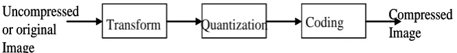
An image, according to [13], is defined as an artifact that shows or records visual perception. Image is a kind of redundant data that contains the same information from certain perspective of view. Hence, by using compression methods, it is possible to remove some of the redundant information contained in images [13]. Irrespective of the image compression method employ, compression method that will guarantee high compression ratio with better accuracy usually involves the basic steps shown in Figure 1. Hence, for a typical lossy image compression method, the first step involved is a mathematical transformation that allows switching from spatial domain to a transform domain where coefficients are low correlated. This step is followed by quantization step while the final step is coding, which produces the stream representing the compressed image.
Figure 1. Typical image compression model.
Generally, two major transforms are usually used in image compression. These two transforms are discrete cosine transform (DCT) and discrete wavelet transform (DWT). The two transforms use the principle of de-correlation in the first step of Figure 1 to extract relevant information from the image and reduce redundancy in the image. Basically, the method of image compression is not new as discovery of DCT in 1974 motivated study on image compression. Until recently, the DCT as reported in [14] has been the most popular transform technique for compression as a result of its optimal performance and ability to be implemented at a reasonable cost. Some of the popular emerged standards that employed DCT algorithm or principle in image compression are the Joint Photographic Experts Group (JPEG) [15], Moving Picture Expert Group (MPEG) [16] and Px64 [17]. While JPEG is being used for compression of photograph and still images, MPEG and Px64 are used for compression of motion video, and video telephony and teleconferencing respectively.
However, as reported in [18], a fundamental shift in image compression scheme came after the DWT became popular. This popularity as well as DWT inherit multi-resolution nature aids its widespread acceptance in signal processing and image compression. On the other hand, in 1996, according to [5], Said and Pearlman developed wavelet based image compression algorithm known as set partitioning in hierarchical tree (SPIHT). The SPIHT uses the principle of zero-tree coding from embedded zerotree wavelet (EZW) as well as wavelet decomposition and imposes a quad tree structure across the sub-bands in order to exploit the inter-band correlation. The algorithm uses a special data structure called spatial orientation trees (SOT) instead of an arithmetic encoder with better and efficient compression performance. Brief review on each of these three image compression (DCT, DWT and SPIHT) algorithms employed in this study and their procedural steps are presented in the following subsections.
Transform Quantization Coding Uncompressed
or original Image
Compressed Image Transform Quantization Coding
Uncompressed or original Image
2.1. Discrete cosine transform algorithm
Basically, there are two types of discrete cosine transform (DCT), namely one dimensional DCT and two dimensional DCT. While the one dimensional DCT is used for processing one-dimensional signals such as speech waveform, the two-dimensional (2D) DCT is used for analyzing signals such as images. Irrespective of the DCT type use, the DCT compression algorithm or technique works by transforming image from spatial domain to the frequency domain. It does the image transformation process by separating the image into spectral sub-bands of differing importance in respect to the image’s visual quality. This is achieved by representing the uncompressed or original image points in the form of sum of cosine functions that are oscillating at different frequencies and magnitudes.
Hence, in this study, which is on image compression, the 2D DCT for an NxN input was employed. The 2D DCT employed is defined mathematically in [19] as;
j
N
y
i
N
x
y
x
M
j
B
i
B
N
j
i
D
N x N y DCT2
1
2
cos
2
1
2
cos
.
,
2
1
,
1 0 1 0 (1)where
M
x
,
y
is the input image of sizex
y
,
0 , 1 0 , 2 1 i if i if iB and
0 , 1 0 , 2 1 j if j if j B .
In this study, the input image is first divided into 88 blocks and the 8-point 2D DCT is performed. The DCT coefficients, according to [19], are then quantized using 88 quantization. The quantization is attained by dividing each elements of the transformed input image matrix by corresponding element in the quantization matrix Q and rounding to the nearest integer value using the mathematical expression given in [19] as;
j
i
Q
j
i
D
round
j
i
D
DCT quant,
,
,
(2)where
ij i j i i i j i j i i i j j j jq
q
q
q
q
q
q
q
q
q
q
q
q
q
q
q
j
i
Q
2 1 1 1 1 2 1 1 1 2 1 2 22 21 1 1 1 12 11,
(3)factor. The quantized coefficients are then rearranged in a zigzag order, as reported in [20], to further compress the image by an efficient lossy coding algorithm.
The four basic activities or procedures involved in DCT image compression is summarized as follows: Firstly, the uncompressed image to be compressed is broken into NN blocks, where
. , 4 , 3 , 2 ;
2 n etc
N n Secondly, the DCT is applied to each block working from left to right and top to bottom. Thirdly, each block’s element is compressed through quantization means. Lastly, the array of compressed blocks that constitute image is stored in a drastically reduced amount of space.
2.2. Discrete wavelet transform algorithm
In discrete wavelet transform (DWT), an uncompressed image is represented by sum of wavelet functions, which are known as wavelets. These wavelets have different locations and scales. Basically DWT represents the image to be compressed into a set of high pass coefficients called details and low pass coefficients also known as approximates. The uncompressed or original image is first divided into NNblocks, where N32. Each block is then passed through two filters [19]. In the first filter, decomposition is performed to decompose the input image into detail and approximate coefficients. The obtained detail and approximate coefficients are then separated into LLn, HLn, LHn
and HHn coefficients where LLn is low pass filter over rows and columns, HLn is high pass filter over
rows and low pass filter over columns, LHn is low pass filter over rows and high pass filter over
columns and HHn is high pass filter over rows and over columns. The result, according to [21], is a
four sub-band term LL1 (horizontally and vertically low pass), HL1 (horizontally high pass and
vertically low pass), LH1 (horizontally low pass and vertically high pass) and HH1 (horizontally and
vertically high pass). In order to increase the efficiency of the DWT, multiple decomposition stage is recursively performed on the LL1 sub-band to smoothed version of the original image. Thus LL1 is
decomposed to LL2, HL2, LH2 and HH2 as shown in Figure 2.
Figure 2. An image of 3-level 2D DWT decomposition [21].
Generally, the basic procedures involved in DWT image compression are summarized as follows: Firstly, a wavelet is chosen. Then choose decomposition level N and compute the wavelet. Secondly, for each level from 1 to N, a threshold is decided and applied to the detail coefficients. Finally, wavelet reconstruction is computed using the original approximation coefficients of level N and the modified detail coefficients of levels from 1 to N.
LL3 HL3
HH3
LH3
HL2
LH2 HH2
HL2
HH1
LH1
LL3 HL3
HH3
LH3
HL2
LH2 HH2
HL2
HH1
2.3. Set partitioning in hierarchical tree algorithm
The set partitioning in hierarchical tree (SPIHT), according to [5], uses wavelet sub-band decomposition and imposes a quad tree structure across the sub-bands in order to exploit the inter-band correlation. The algorithm according to [5], searches each tree, and partitions the tree into one of these three lists: one, the list of significant pixels (LSP) containing the coordinates of pixels found to be significant at the current threshold; two, the list of insignificant pixels (LIP), with pixels that are not significant at the current threshold; and three, the list of insignificant sets (LIS), which contain information about trees that have all the constituent entries to be insignificant at the current threshold. Figure 3 shows the tree structure for level 2 decomposition in SPIHT algorithm.
Figure 3. Tree structure used in SPIHT algorithm [5].
Basically, the procedures involved in SPIHT image compression algorithm is divided into three stages, namely: initialization, sorting pass and refinement pass. The activities involved in each stage are summarized as follows: Firstly, at the initialization stage, a start threshold is defined by the algorithm according to the maximum value in the wavelet coefficients pyramid and sets the LSP as an empty list and puts the coordinates of all coefficients in the coarsest level of the wavelet pyramid (LL
band) in the LIP and those which have descendants to the LIS. Secondly, at the sorting pass, features in the LIP and the LIS are sorted. Significance test is carried out on each pixel in LIP matched against the current threshold and outputs the test result (0 or 1) to the output bit-stream. For significant coefficient, its coordinate is moved to the LSP. The sorting pass of LIS, SPIHT does the significant test for each set in the LIS and outputs the significance information (0 or 1). If a set is significant, it is partitioned into its offspring and leaves. The current threshold is divided by 2. Finally, according to [22], the sorting and refinement stages are continued until target bit-rate is achieved.
3. Methodology
In carrying out this study, the uncompressed or original images used for the study were acquired using smart-camera. The acquired images were then stored on secured digital or memory card of the camera and consequently transferred to the memory of the computer used. This is to enhance easy accessibility to the images as well as to allow further processing on the images such as extraction of
LL1 HL2
LH2 HH2
HL1
HH1 LH1
LL1 HL2
LH2 HH2
HL1
some features from the acquired images. The information extracted includes the image size, format, color depth, alignment and color. This extraction process serves as a prelude to the compression process. MATLAB function was written to get the details of the images. Also, MATLAB functions were developed for the three image compression algorithms reviewed in last section. The image compression process was then carried out in MATLAB environment. The acquired uncompressed images were compressed using each of the three algorithms developed. After the successful development of the three image compression algorithms, the performance of each of them was evaluated.
In carrying out the performance evaluation of the three algorithms, five performance indices were employed. The five performance indices employed as mentioned earlier are peak-signal-to-noise-ratio (PSNR), mean square error (MSE), compression ratio (CR), algorithm operating time and image histogram. PSNR is a measure of peak error in compressed image. It is the most commonly used performance index to measure the quality of reconstruction of lossy image compression. It is evaluated in decibel using the mathematical expression defined in [19] as;
MSE
I
PSNR
2 10
log
10
(4)where
I
is a constant known as allowable image pixel intensity level. On the other hand, MSE is the cumulative squared error between the compressed image and the original or uncompressed image. It is defined mathematically in [23,24] as;
Mx N
y
y
x
f
y
x
f
MN
MSE
1 1
2
,
ˆ
,
1
(5)
where
f
x
,
y
is the original image, fˆ
x,y is the compressed image, M and N are the matrix dimensions inx
and y respectively. Basically, PSNR and MSE are the two error matrices usually used to compare compression quality. Technically, the higher the value of PSNR, the better the quality of the obtained compressed image.Compression ratio (CR), on the other hand, is an engineering term used to quantify the reduction in image size produced by image compression algorithm. It is the ratio of the original image size to that of the compressed image. It is defined in [24] as the nominal bit depth of the original image in bits per pixel divided by the bits per pixel necessary to store the compressed image. It is expressed mathematically in [23] as;
2 1
n n
CR (6)
where
n
1 andn
2 are the original size or number of bits in original image and the compressed imagealgorithm operating time. This gives the time taken for the each algorithm to compress a specific image. The results obtained when the three developed image compressed algorithms were evaluated using the five performance indices are presented and discussed in next section.
4. Experimental Results and Discussion
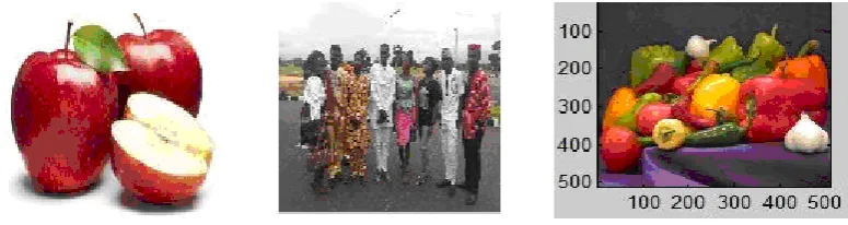
After the successful development of the three image-compression algorithms, their respective efficiency in image compression capability were evaluated using the five performance indices described above. The three original images used in evaluating the performance of the three developed image compression algorithms are shown in Figure 4. The results obtained in each case are presented and discussed in the following subsections.
Figure 4. Original images for the performance evaluation analysis.
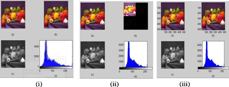
4.1. The algorithms performance evaluation using image histogram
Figure 5. (i) DCT, (ii) DWT and (iii) SPIHT performance evaluations results for apple.
Figure 6. (i) DCT, (ii) DWT and (iii) SPIHT performance evaluations results for picture.
Figure 7. (i) DCT, (ii) DWT and (iii) SPIHT performance evaluations results for pepper.
(i) (ii) (iii)
(i) (ii) (iii)
(i) (ii) (iii)
(i) (ii) (iii)
(i) (ii) (iii)
(i) (ii) (iii)
(i) (ii) (iii)
(i) (ii) (iii)
4.2. The algorithms performance evaluation using compression ratio (CR)
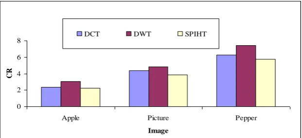
CR as defined above is a compression performance index that quantifies the reduction in image size produced by image compression algorithm. Hence, the higher the CR value obtained from an image compressing algorithm, the better the algorithm that produces it. Thus, as shown in Figure 8, DWT algorithm outperforms the two other algorithms while SPIHT directly follows DWT and DCT is the last for the three images used in evaluating the performance of the three developed image compression algorithm.
Figure 8. CR comparative performance results for the three algorithms.
4.3. The algorithms performance evaluation using PSNR and MSE
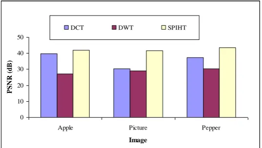
Furthermore, in assessing the comparative performance evaluations of the three developed image compression algorithms for this study, MSE and PSNR, which are two of the most popular performance indices to estimate the efficiency and effectiveness of image compressing algorithm, were employed using the three original images as test samples. The experimental results obtained for MSE and PSNR are presented graphically in Figures 9 and Figure 10 respectively. From the results presented in Figure 9 and Figure 10 as well as equation (4), it is obvious that there is inverse proportionality relationship between MSE and PSNR. Hence, from the observations of the experimental results of PSNR and MSE, it is deduced that when assessing the reconstructed images under these performance indices, SPIHT showed good performance throughout with better quality of images at the same time. Therefore, it can be established that SPIHT is the best algorithm based on the experimental results of this study. This inference is justified on MSE result in Figure 9 as errors introduced in those images by DWT and DCT algorithms for each image is relatively higher than the corresponding error introduced by SPIHT algorithm. Therefore, since the higher the MSE value the higher the distortional value introduced, it is obvious that only SPIHT algorithm reproduced the sample images with minimal distortion level.
0 2 4 6 8
Apple Picture Pepper
Image
CR
Figure 9. MSE comparative performance results for the three algorithms.
Figure 10. PSNR comparative performance results for the three algorithms.
4.4. The algorithms performance evaluation using operating time and compression distortion
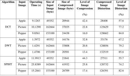
Critical observations of Table 1 show that DWT algorithm has least computational complex. On the other hand, DCT and SPIHT algorithms are relatively more computational complex than DWT algorithm. This accounts for the reason why the operating time for SPIHT is the highest for the same input image while that of the DWT is the lowest with that of DCT in between them. In addition, Table 1 shows that for the same input image DWT algorithm has the least percentage level of image compression among the three algorithms. Furthermore, critical observations of Figure 9 and Table 1 show that DWT algorithm gives considerably highest distortion in image compression size follows by DCT algorithm while SPIHT algorithm gives the lowest. Hence, with the this highest level of distortion by DWT algorithm as shown in Figure 9 and buttresses numerically in Table 1, SPIHT is found to be the best among the three algorithms because of its comparably better image compression quality and minimal distortion level advantage while DWT algorithm is the least and DCT algorithm is between the two extremists for the same reason.
0 10 20 30 40 50
Apple Picture Pepper
Image
P
S
N
R
(
d
B
)
DCT DWT SPIHT
0 20 40 60 80 100 120 140
Apple Picture Pepper
Image
M
S
E
Table 1. Developed algorithms comparative analysis in terms of complexity and distortion
Algorithm Input Image
Operating Time (s)
Size of Input Image (byte)
Size of Compressed Image (byte)
Level of Image Compression
(%)
Compressed Image Distortion
Level of Image Distortion
(%)
DCT
Apple 9.1263 49352 20944 42.4 28408 57.6
Picture 10.1290 162664 37035 22.8 125629 77.2
Pepper 9.8561 153100 24438 16.0 128662 84.0
DWT
Apple 1.3972 49352 16176 32.8 33176 67.2
Picture 1.4291 162664 33808 20.8 128856 79.2
Pepper 1.4706 153100 20581 13.4 132519 85.6
SPIHT
Apple 11.9913 49352 21841 44.3 27511 55.7
Picture 25.8389 162664 41932 25.8 120732 74.2
Pepper 15.2841 153100 26709 17.4 126391 82.6
5. Conclusion
This study presents three developed image compression algorithms. The performance evaluations of the three developed algorithms were determined using five performance indices. The results of the performance evaluations conducted show that the three developed algorithms performed favorably well with varying compression ratios and different qualities of images. Also, the results of the performance evaluations of the three developed algorithms show that the three algorithms are effective in image compression capability though with different efficiency values. Furthermore, the experimental results of the computational distortional analysis conducted on the three developed image compression algorithms show that SPIHT algorithm has minimal distortion level followed by DCT algorithm, while DWT algorithm has the highest distortional percentage value. Hence, in terms of image size reduction, DWT algorithm is the best among the three algorithms followed by DCT algorithm while SPIHT algorithm is the last. However, since the objective of this study is to determine the best algorithm with minimal distortional value among the three algorithms, it therefore concludes base on the obtained results that SPIHT algorithm is the best followed by DCT while DWT algorithm is the last.
References
[1] Singh, Singh, A.K. and Tripathi, G.S. (2014). A Comparative Study of DCT, DWR and hybrid (DCT-DWT) Transform, GJESER Review Paper, Vol. 1, No. 4, pp. 16-21.
[2] Dhawan, S. (2011). A Review of Image Compression and Comparison of its Algorithms, International Journal of Electronics and Communication Technology, Vol. 2, No. 1, pp. 22-26.
[3] Gupta, B. (2013). Study of Various Lossless Image Compression Techniques, International Journal of Emergimg Trends and Technology in Computer Science, Vol. 2, No. 4, pp. 253-257.
[4] Rehman, M., Sharif, M. and Raza, M. (2014). Image Compression: A Survey, Research Journal of Applied Sciences, Engineering and Technology, Vol. 7, No. 4, pp. 256-672.
[5] Nivedita, M. Singh, P., and Jindal, S. (2012). A Comparative Study of DCT And DWT-SPIHT.
International Journal of Computational Engineering and Management, Vol. 15, No. 2, pp. 26-32.
[6] Pensiri, F. and Auwatanamongkol, S. (2012). A Lossless Image Compression Algorithm Using Predictive Coding Based on Quantized Colors, WSEAS Transactions on Signal Processing, Vol. 8, No. 2, pp. 43-53. [7] Alarabeyyat, A., Al-Hashemi S., Khdour, T., Btoush, M.H., Bani-Ahmad, S. and Al-Hashemi, R. (2012),
Lossless Image Compression Technique Using Combination Methods, Journal of Software Engineering and Applications, Vol. 5, pp. 752-763.
[8] Weinberger, M.J., Seroussi, G. and Sapiro, G. (2000). The LOCO-I Lossless Image Compression Algorithm: Principles and Standardization into JPEG-LS, IEEE Trans. on Image Processing, Vol. 9, No. 8, pp. 1309-1324.
[9] Zuo, Z., Lan, X., Deng, L., Yao, S. and Wang, X. (2015). An Improved Medical Image Compression Technique with Lossless Region of Interest. Optik-International Journal for Light and Electron Optics, Vol. 126, No. 21, pp. 2825-2831.
[10] Tomar, R.R.S. and Jain, K. (2016). Lossless Image Compression Using Differential Pulse Code Modulation and its Application, International Journal of Signal Processing, Image Processing and Pattern Recognition, Vol. 9, No. 1, pp. 197-202.
[11] Masood, S., Sherif, M., Yasmin, M., Raza, M. and Mohsin, S. (2012). Brain Image Compression: A Brief Survey. Research Journal of Applied Sciences, Engineering and Technology, Vol. 5, No. 1, pp. 49-59. [12] Marimuthu, M., Muthaiah, R. and Swaminathan, P. (2012). Review Article: An Overview of Image
Compression Techniques. Research Journal of Applied Sciences, Engineering and Technology, Vol. 4, No. 24, pp. 5381-5386.
[13] Vijayvargiya, G., Silakari, S. and Pandy, R. (2013). A Survey: Various Techniques of Image Compression.
International Journal of Computer and Information Security, Vol. 11, No. 10, pp. 51-55.
[14] Rehna, V.J.and Jeya Kumar, M.K. (2012). Wavelet Based Image Coding Schemes: A Recent Survey,
International Journal of Soft Computing, Vol. 3, No. 3, pp. 101-118.
[15] Wallace, G.K. (1991). The JPEG Still Picture Compression Standard, Communications of the ACM Magazine, Vol. 34, No. 4, pp. 30-44.
[16] Puri, A. (1992). Video Coding Using the MPEG-1 Compression Standard, Society for Information Display Digest of Technical Papers, Vol. 23, pp. 123-126.
[17] Watson, A.B. (1994). Image Compression Using the Discrete Cosine Transform, Mathematica Journal, Vol. 4, No. 1, pp. 81-88.
[18] Yadavi, R.J., Gangwar, S.P. and Singh, H.V. (2012). Study and Analysis of Wavelet Based Image Compression Techniques International Journal of Engineering, Science and Technology, Vol. 4, No. 1, pp. 1-7.
[19] Bindu, K., Ganpati, A. and Sharma, A.K. (2012). A Comparative Study of Image Compression Algorithms,
International Journal of Research in Computer Science, Vol. 2, No. 5, pp. 37-42.
[21] Al-Janabi, A.K. (2013). Low Memory Set-Partitioning in Hierarchical Trees Image Compression Algorithm, International Journal of Video and Image Processing and Network Security, Vol. 13, No. 2, pp. 12-18.
[22] Rema, N.R., Binu A.O. and Mythili, P. (2015). Image Compression Using SPIHT with Modified Spatial Orientation Tress, Procedia Computer Science, Vol. 46, pp. 1732-1738.
[23] Chowdhury, M.M.H. and Khatun, A. (2012). Image Compression Using Discrete Wavelet Transform,
International Journal of Computer Science Issues, Vol. 9, No. 1, pp. 327-330.
![Figure 2. An image of 3-level 2D DWT decomposition [21].](https://thumb-us.123doks.com/thumbv2/123dok_us/8774762.1758886/5.595.222.376.470.601/figure-image-level-d-dwt-decomposition.webp)
![Figure 3. Tree structure used in SPIHT algorithm [5].](https://thumb-us.123doks.com/thumbv2/123dok_us/8774762.1758886/6.595.203.357.262.417/figure-tree-structure-used-spiht-algorithm.webp)