ISSN: 2008-6822 (electronic)
http://dx.doi.org/10.22075/ijnaa.2015.222
Wavelet collocation solution of non-linear Fin problem with
temperature dependent thermal conductivity and heat transfer
coefficient
Surjan Singha,∗, Dinesh Kumara, K. N Raib
aDST- Centre for Interdisciplinary Mathematical Sciences Banaras Hindu University Varanasi 221005, U.P., India
bDepartment of Mathematical Science IIT BHU, Varanasi 221005, India
(Communicated by M. Eshaghi Gordji)
Abstract
In this paper, Wavelet Collocation Method has been used to solve nonlinear fin problem with temperature dependent thermal conductivity and heat transfer coefficient. Thermal conductivity of fin materials varies any type so that we consider thermal conductivity as the general function of temperature. Here we consider three particular cases, where we assume that thermal conductivity is constant, linear and exponential function of temperature. In each case efficiency of fin is evaluated. The whole analysis is presented in dimensionless form and the effect of variability of fin parameter, exponent and thermal conductivity parameter on temperature distribution and fin efficiency is shown graphically and discussed in detail.
Keywords: Collocation; conductivity; fin, temperature; transfer; wavelet.
MSC:Primary 34B15; Secondary 34G20.
1. Introduction and preliminaries
Nomenclature:
Ac = cross section area of the fin (m2) exp = exponential term
h= heat transfer coefficient (W m−2K−1)
hb = the heat transfer coefficient at fin base (W m−2K−1) k= thermal conductivity of fin material (W m−1K−1)
ka = thermal conductivity at ambient temperature(W m−1K−1) L= length of fin (m)
n= exponent
P = perimeter of the fin (m)
T = local temperature on the fin surface (K) Ta = environment (ambient ) temperature (K)
∗Corresponding author
Email addresses: [email protected](Surjan Singh),[email protected] (Dinesh Kumar),[email protected] (K. N Rai)
Tb= base temperature of the fin (K) x= dimensional space coordinate (m)
λ= the slope of the thermal conductivity-temperature curve (K−1) η = fin efficiency
Dimensionless variables and similarity criteria
N =qhbP L2
kaAc fin parameter
X= Lx space coordinate, θ= (T−Ta
Tb−Ta) temperature of the fin
β=λ(Tb−Ta),
Abbreviation
ADM = Adomian Decomposition Method HAM = Homotopy Analysis Method HPM = Homotopy Perturbation Method WCM = Wavelet Collocation Method
Heat exchangers are known as fins. In the study of heat transfer, fin is the surface made by metallic material which is used to increase the rate of heat transfer to environment. The rate of heat transfer depends on the surface area of the fin. Heat transfer is most important aspect in industrial processes. In industry, heat is removed for smooth functioning of machine, for that it is either added or transfered from one medium to another.
Medium chosen may be liquid, solid or gas. Fin or heat exchangers are widely used in industries, for instance in sugar plants, chemical plants, power plants, refineries, Automobile industry, food, medical science, petroleum, air conditioning, refrigeration, chilling plant, cold storage etc. and electrical devices like motors and transformers in which the generated heat can be efficiently transferred. Typically, the fin material has a high thermal conductivity. The most common fin materials are aluminium alloys. Aluminium alloys 6061 and 6063 are commonly used, with thermal conductivity values of 166 and 201 W/m K, respectively. Copper has around twice the conductivity of aluminium, and five times more expensive than aluminium. Diamond is another heat sink material and its thermal conductivity is 2000 W/mK which exceeds copper by five-folds. In contrast to metals, where heat is conducted by delocalized electrons, lattice vibrations are responsible for diamond’s very high thermal conductivity. Composite materials can also be used; for example a copper-tungsten pseudo-alloy, AlSiC (silicon carbide in aluminium), Dym-alloy (diamond in copper-silver alloy) etc. For production of heat exchangers copper, cast steel, aluminium metals are generally used. Silver has highest thermal conductivity of all the known metals at room temperature.
problem for a single fin or spine of constant cross section with an insulated tip is generalized to account for the effect of the tip heat loss.
Min-Hsing Chang [3] used ADM to analyze the thermal characteristics of a straight rectangular annular fin for all possible types of heat transfer. This method provides a simple approximate solution. Operational matrix of integration presented by M. Razzaghi et al.[15]. M.S.H. Chowdhury et al.[5] the power-law fin-type problem was solved by the Homotopy Analysis Method and the result thus obtained is compared with the exact solution and decomposition method. The obtained solutions are more accurate with easily computable terms. Sazzad Hossien Chowdhury [6] used HPM to evaluate temperature distribution in fin, where heat transfer coefficient is considered to vary with a power-law type function of temperature. He compared his results for thirteen-terms ADM solution and six-term modified HPM, here HPM gives better result. Rafael Cortell [7] used numerical analysis to obtain the temperature distribution within a single fin. It is assumed that the heat transfer coefficient depends on temperature and is considered as power law type form. S. Abbasbandy and E. Shivanian [1] found an exact analytical solution in implicit form of a nonlinear equation for different values ofn; and obtained dual solutions forn =−3/2, N =±0.9 and n=−3, N =±0.4.Sin Kim and Huang [13] provide an extension of a series solution of this nonlinear fin problem. It has been shown that the Adomian decomposition solution is just an approximation of the series solution given in their work. The accuracy of approximate solution is verified with the numerical solution. In difficult nonlinear moving fin problem, Legendre wavelet basis functions and WCM method is used by [17]. In [17], thermal conductivity of fin is considered as constant or a linear function of temperature. No solution is available when thermal conductivity of fin varies with temperature in general.
In this study we consider the heat transfer in a fin whose thermal conductivity varies in general with temperature and the heat transfer coefficient is expressed as a power law type form. To solve this nonlinear boundary value problem, we use Wavelet Collocation Method (WCM).
As WCM require less computation and provide better result in comparison to other methods. Three particular cases namely when thermal conductivity is (I) constant, (II) linear and (III) exponential function of temperature are discussed in detail.
2. Formulation of the problem
We consider straight one dimensional fin with a constant cross section areaAc. The fin, with perimeterP and length L, is attached to a base surface of temperature Tb and extends into a fluid of temperature Ta. It is assumed that the amount of heat transfer through the tip end is negligibly small. The one dimensional steady-state heat balance equation can be written as
Ac d dx
k(T)dT dx
−P h(T−Ta) = 0, 0< x < L, (2.1)
with conditions
x= 0,dT dx = 0 x=L, T=Tb
wherehis the heat transfer coefficient and may be non-uniform along the fin.
The heat transfer coefficient may depend on the temperature and usually can be expressed as a power form
h=h(T) =hb
T−T a Tb−Ta
n
, (2.2)
wherehb is the heat transfer coefficient at the base temperature. The exponentndepends on the heat transfer mode. Typical values of n are -1/4 for laminar film boiling or condensation, 1/4 for laminar natural convection, 1/3 for turbulent natural convection, 2 for nucleate boiling, 3 for radiation and 0 for constant heat transfer coefficient. In Eq. (2.1), K is the thermal conductivity. We consider thermal conductivity as the general function of temperature i.e.
k(T) =kaf T
−Ta Tb−Ta
.
Introducing the dimensionless variables
θ= T−Ta Tb−Ta
, X= x
L, β=λ(Tb−Ta), N
2= hbP L2 kaAc
The heat balance Eq. (2.1) can be written as
f(θ)d
2θ
dX2 +g(θ)
dθ dX
2
−N2θn+1= 0. (2.4)
The Eq. (2.4) is subjected to
θ0(0) = 0 (2.5)
θ(1) = 1 (2.6)
3. Solution of the problem
We solve this problem using Wavelet Collocation Method. Continuous Wavelets is defined by the following formula
ψa,b(X) =|a|
−1 2 ψ
X−b
a
, a, b∈R, a6= 0, (3.1)
whereais dilation parameter andb is a translation parameter. Legendre wavelets is defined on the interval (0,1) by [15]
ψn,m(X) = (p
(m+ 1/2)2k/2Pm 2kX−nˆ
, nˆ2−1k ≤X ≤
ˆ n+1
2k
0 , otherwise , (3.2)
wherem= 0,1, . . . , M−1 andn= 1,2, . . . ,2k−1.HerePm(X) is the well known Legendre polynomials of order m.
P0(X) = 1, P1(X) =X, Pm+1(X) =
2m+ 1
m+ 1 XPm(X)− m
m+ 1Pm−1(X), m= 1,2,3, . . . , M−1. (3.3) A function f(X) defined in domain [0,1] can be expressed as
f(X) =
∞ X n=1 ∞ X m=0
cn,mψn,m(X), (3.4)
wherecn,m=< f(X), ψn,m(X)>in which < ., . >denotes the inner product. If we take some terms of infinite series, then Eq. (3.4)can be written as
f(X) =
2k−1
X
n=1 M−1
X
m=0
cn,mψn,m(X) =CTψ(X), (3.5)
where C andψ(X)are M ×1 Matrices given by
C= [c1,0, c1,1, . . . , c1,M−1, c2,0, c2,1, . . . , c2,M−1, c2k−1,0c2k−1,1, . . . , c2k−1,M−1]T. (3.6)
ψ(X) = [ψ1,0(X), ψ1,1(X), . . . , ψ1,M−1(X), ψ2,0(X), . . . , ψ2,M−1(X), . . .
ψ2k−1,0(X)ψ2k−1,1(X), . . . , ψ2k−1,M−1(X)]T. (3.7)
(i)Property of the product of two Legendre wavelets
If E is a given wavelets vector then we have the property
ETψψT =ψTE,ˆ (3.8)
where ˆE is M×M matrices depend on the wavelet vectorE.
(ii) Operational matrix of integration
The integration of the waveletsψ(X) which is defined in Eq. (3.2) can be obtained as
X Z
0
whereP isM×M operational matrix of integration is given by
P =1 2
1 √1
3 0 · · · 0 −1
√ 3 0
1 √
15 · · · 0
0 √−1
15 0 · · · 0
..
. . .. ...
0 0 0 · · ·
√ 2M−3 (2M−3)√2M−1
0 0 0 · · · −
√ 2M−3 (2M−3)√2M−1 0
. (3.10)
3.1. Wavelet Collocation Method
Let
θ00(X) =CTψ(X). (3.11)
Integrating from 0 to X, we get
θ0(X) =θ0(0) +CTP ψ(x),
⇒θ0(X) =CTP ψ(X). (3.12)
Again integrating above equation and using boundary conditions Eq. (2.5)and Eq. (2.6), we get
θ(X) =θ(0) +CTP2ψ(X). (3.13)
Putting X = 1 in Eq. (3.13), we get
θ(0) = 1−CTP2ψ(1).
Substitutingθ(0) in Eq. (3.13), we get
θ(X) = 1−CTP2ψ(1) +CTP2ψ(X). (3.14)
Substituting the value ofθ00(X) andθ(X) in Eq. (2.4), we obtain
f(θ)CTψ(X) +g(θ)(CTP ψ(X))2−N2
1−CTP2ψ(1) +CTP2ψ(X) n+1
=R(X, c1, c2, . . . , cn) = 0. (3.15)
Asθ(X) is an approximate solution of system Eq. (2.4) to Eq. (2.6). Choosing n collocation pointsXi, i= 1,2,3, . . . , n in the interval (0,1),at which residualR(X, c1, c2, . . . , cn) equal to zero. The number of such points must be equal to the number of coefficientsci, i= 1,2,3, . . . , n. Thus, we getR(X, c1, c2, . . . , cn) = 0, i= 1,2,3, . . . , n.
Here we consider three particular cases as follows:
Case IThermal conductivity is constant,k=ka i.ef(θ) = 1, g(θ) = 0.Eq. (3.15) reduces to CTψ(X)−N2{1−CTP2ψ(1) +CTP2ψ(X)}n+1=R(X, c
1, c2, . . . , cn). (3.16)
Case IIThermal conductivity is the linear function of temperature,
k=ka{1 +λ(T−Ta)}i.e.f(θ) = 1 +βθ, g(θ) =β.
Eq. (3.15) takes the form
1 +β
1−CTP2ψ(1) +CTP2ψ(X) CTψ(X) +β
CTP ψ(X) 2
−N2{1−CTP2ψ(1) +CTP2ψ(X)}n+1=R(X, c
1, c2, . . . , cn). (3.17)
Case IIIThermal conductivity is exponential function of temperature,
k=kaeλ(T−Ta)i.e.f(θ) =eβθ, g(θ) =βeβθ, Eq. (3.15) becomes
eβ{1−CTP2ψ(1)+CTP2ψ(X)}CTψ(X) +βeβ{1−CTP2ψ(1)+CTP2ψ(X)}CTψ(X)CTP ψ(X) 2
−N2{1−CTP2ψ(1) +CTP2ψ(X)}n+1=R(X, c1, c2, . . . , cn). (3.18)
4. Fin Efficiency
The fin efficiency is the ratio of actual heat transferred from the fin surface to the surrounding fluid; to the heat conducted through the base atX =L (orX = 1). The efficiency can be written as
η= kAC dT dx|x=L P h(Tb−Ta)L
. (4.1)
In Case I efficiency
η= 1 N2θ
0(1), f orN6= 0, N= 1,2,3,4,5. (4.2)
In Case II efficiency
η=1 +β N2 θ
0(1). (4.3)
In Case III efficiency
η= e β
N2θ
0(1). (4.4)
5. Results and discussion
The value of exponent n depends on the heat transfer mode. We choose three values (−1/4,1/3,3) of exponent n for laminar film boiling or condensation, turbulent natural convection and radiation respectively. Temperature distribution in fin depends on fin parameter N, β and exponent n. We use nine Legendre wavelet basis functions in computation. For constant thermal conductivity (β = 0) temperature distribution in fin decreases as N increases, shown in Figure 2. In Table 1 we compare wavelet collocation method and exact results, both are same for N = 0.5 andN = 1 and it proves the accuracy of the method.
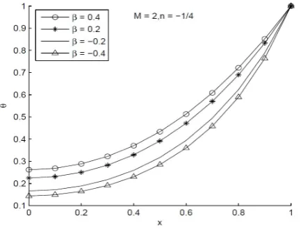
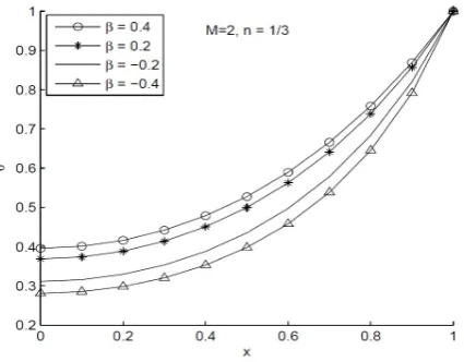
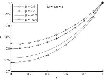
The result thus obtained is correct up to ten decimal places forN = 0.5 and 1. In Case II and III the dimensionless temperature distributions along the fin surface when β vary from -0.4 to 0.4 and n vary from -1/4, 1/3 to 3 are presented in Figures 3 to 14 forN = 1 andN = 2. For laminar film boiling or condensation (n=−1/4) andN = 1 temperature in fin increases asβ increases in Case II and III both, but temperature in Case III is always higher than Case II as shown in Figures3 and 4. Forn=−1/4 andN = 2 temperature distribution in fin increases asβ increases in Case II and III which is presented in Figures 5 and 6. For turbulent natural convection (n= 1/3) and N = 1,2 temperature distribution in fin increases asβ increases in Case II and III both and is presented by Figures 7, to10. In turbulent natural convection we observe that forN = 1, n= 1/3 andβ = 0.4,temperature atX = 0 in fin is 0.7343, 0.7439 in Case II and III respectively. ForN = 2, n= 1/3 andβ = 0.4,temperature atX = 0 in fin is 0.3958, 0.4041 in Case II and III respectively. In radiation mode (n= 3) temperature atX = 0 in fin forN = 1 is 0.8134, 0.8191 and forN = 2 is 0.6400, 0.6457 in Case II and III respectively. Thus, temperature in fin atX = 0 increases for laminar film boiling (or condensation) to turbulent natural convection and from turbulent natural convection to radiation. It has been observed that the heat transfer through fin is highest in radiation mode. In Case III, temperature distribution in fin is always higher than Case II as shown in Figures 3 to 14. Summary of minimum and maximum temperature distribution in fin atX= 0 is given in Table2 for Case I, II and III.
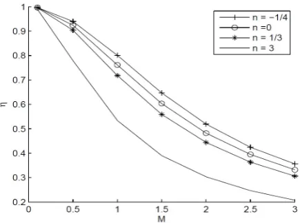
Fin efficiency is presented in Figures15 to 18 for different values ofn, β, andN. In Case I effect ofnandN on fin efficiency is shown in Figure15. It is clear from this figure that fin efficiency decreases as the value ofnincrease from -1/4 to 3 andN increases from 0 to 3. In this case the fin efficiency is higher for laminar film boiling or condensation (n=−1/4).
Table 1: The dimensionless temperature distribution in case of constant thermal conductivity (β= 0)
N=0.5 N=0.5 N=1 N=1
X Exact WCM Exact WCM
0.0 0.8868188840 0.8868188840 0.6480542737 0.6480542737 0.1 0.8879276385 0.8879276385 0.6512972462 0.6512972462 0.2 0.8912566747 0.8912566747 0.6610586204 0.6610586204 0.3 0.8968143168 0.8968143168 0.6774360915 0.6774360915 0.4 0.9046144618 0.9046144618 0.7005935707 0.7005935707 0.5 0.9146766141 0.9146766141 0.7307628258 0.7307628259 0.6 0.9270259345 0.9270259345 0.7682458010 0.7682458010 0.7 0.9416933025 0.9416933025 0.8134176383 0.8134176383 0.8 0.9587153943 0.9587153943 0.8667304327 0.8667304327 0.9 0.9781347739 0.9781347739 0.9287177566 0.9287177566 1.0 1.0000000000 1.0000000000 1.0000000000 1.0000000000
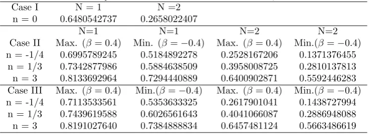
Table 2: Temperature distribution in fin atX= 0 in case I, II and III
Case I N = 1 N =2
n = 0 0.6480542737 0.2658022407
N=1 N=1 N=2 N=2
Case II Max. (β= 0.4) Min. (β=−0.4) Max. (β= 0.4) Min.(β =−0.4) n = -1/4 0.6995789245 0.5184892278 0.2528167206 0.1371376455
n = 1/3 0.7342877986 0.5884638509 0.3958008725 0.2810137813 n = 3 0.8133692964 0.7294440889 0.6400902871 0.5592446283 Case III Max. (β= 0.4) Min.(β =−0.4) Max. (β= 0.4) Min.(β =−0.4) n = -1/4 0.7113533561 0.5353633325 0.2617901041 0.1438727994
Figure 1: Geometry of a straight fin.
Figure 2: Case I, temperature distributions in fin by WCM forn= 0, N= 1,2,3,4,5 top to bottom respectively.
6. Conclusion
1. According to [12] ADM and HPM solutions fails when N increases to a large number but the WCM gives sufficient accuracy for large values ofN.
2. In case I, II and III as we increase the value of fin parameter N, the thermal conductivity decreases and temperature in fin decreases rapidly.
3. Temperature in fin increases with n as given in Figures 3 to 14. The heat transfer through fin is highest in radiation mode (n= 3) and lowest in laminar film boiling or condensation (n=−1/4).
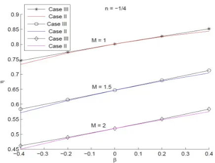
4. In Case II and III, forn=−1/4 fin efficiency decreases asβdecreases from 0 to - 0.4 and increases asβ increases from 0 to 0.4.
5. The fin efficiency increases from Case I to II and II to III (see Figure16). It seems that fin efficiency increases as thermal conductivity of fin material increases with temperature.
A nonlinear straight fin with variable thermal conductivity analysed using the wavelet collocation method. The
Figure 4: Case III, temperature distributions withN= 1 andn=−1/4 forβ=±0.4 andβ=±0.2.
Figure 5: Case II, temperature distributions withN= 2 andn=−1/4 forβ=±0.4 andβ=±0.2.
Figure 7: Case II, temperature distributions withN= 1 andn= 1/3 forβ=±0.4 andβ=±0.2.
Figure 8: Case III, temperature distributions withN= 1 andn= 1/3 forβ=±0.4 andβ=±0.2
Figure 10: Case III, temperature distributions withN= 2 andn= 1/3 forβ=±0.4 andβ=±0.2
Figure 11: Case II, temperature distributions withN= 1 andn= 3 forβ=±0.4 andβ=±0.2.
Figure 13: Case II, temperature distributions withN= 2 andn= 3 forβ=±0.4 andβ=±0.2.
Figure 14: Case III, temperature distributions withN= 2 andn= 3 forβ=±0.4 andβ=±0.2.
Figure 16: Fin efficiency comparison forn=−1/4 in Case I, II and III, variation withN andβ.
Figure 17: Fin efficiency comparison forn= 3 in Case I, II and III, variation withNandβ.
wavelet collocation method is reliable, gives higher accuracy, faster convergence and easy computation. Temperature distribution and efficiency of fin increase from case I to II and case II to III. If we assume the value of n as -1/4, 1/3, 3 temperature in fin increases as given in Figure3 to 14. This method can be applied in difficult nonlinear heat conduction problems, and useful to engineers to analyse nonlinear system.
Acknowledgements
Authors are grateful to Professor Umesh Singh Co-Ordinator DST-CIMS Banaras Hindu University Varanasi, India, for providing necessary facilities. We are thankful to Dr. Satish Kumar, Dept. of English, Gurgaon Institute of Technology and Management Gurgaon (Haryana), India for language editing. The authors express their gratitude to the reviewers for their precious comments, so that technical merit and quality of the paper improved.
References
[1] S. Abbasbandy and E. Shivanian,Exact analytical solution of a nonlinear equation arising in heat transfer, Phys. Lett. A 374 (2010) 567–574.
[2] C. Arslanturk,A decomposition method for fin efficiency of convective straight fins with temperature dependent thermal conductivity, Int. Commun. Heat Mass Transfer 32 (2005) 831–841.
[3] M.H. Chang, A decomposition solution for fins with temperature dependent surface heat flux, Int. J. Heat Mass Transfer 48 (2005) 1819–1824.
[4] C.H. Chiu and C.K. Chen, A decomposition method for solving the convective longitudinal fins with variable thermal conductivity, Int. J. Heat Mass Transfer 45 (2002) 2067–2075.
[5] M.S.H. Chowdhury, I. Hashim and O. Abdulaziz,Comparison of homotopy analysis method and homotopy perturbation method for purely nonlinear fin-type problems, Commun. Nonlinear Sci. Numer. Simul. 14 (2009) 371–378.
[6] M.S.H. Chowdhury,A comparison between the Modified Homotopy perturbation method and adomian decomposition method for solving nonlinear heat transfer Equations, J. Appl. Sci. 11 (2011) 1416–1420.
[7] R. Cortell,A numerical analysis to the nonlinear fin problem, J. Zhejiang Uni. Sci. A9 (2008) 648–653.
[8] G. Domairry and M. Fazeli, Homotopy analysis method to determine the fin efficiency of convective straight fins with temperature dependent thermal conductivity, Commun. Nonlinear Sci. Nonlinear Simul. 14 (2009) 489–499.
[9] I.N. Dul’kin and G.I. Garas’ko,Analytical solutions of the 1-D heat conduction problem for a single fin with temperature dependent heat transfer coefficient-I closed form inverse solution, Int. J. Heat Mass Transfer 45 (2002) 1895–1903.
[10] I.N. Dul’kin and G.I. Garas’ko,Analysis of the 1-D heat conduction problem for a single fin with temperature dependent heat transfer coefficient: part I Extended inverse and direct solutions, Int. J. Heat Mass Transfer 51 (2008) 3309–3324.
[11] D.D. Ganji, Z.Z. Ganji and H.D. Gangi, Determination of temperature distribution for annular fins with temperature dependent thermal conductivity by HPM, Thermal Sci. 15 (2011) S111-S115.
[12] F. Khani, M.A. Raji and H.H. Nejad, Analytical solution and efficiency of the nonlinear fin problem with temperature-dependent thermal conductivity and heat transfer coefficient, Commun. Nolinear Sci. Numer. Simul. 14 (2009) 3327–3338.
[13] S. Kim and C.H. Huang,A series solution of the non-linear fin problem with temperature dependent thermal conductivity and heat transfer coefficient, J. Phys. D Appl. Phys. 40 (2007) 2979–2987.
[14] E. Momoniat, A comparison of two formulations of the fin efficiency for straight fins, Acta Mech. Sin 28 (2012) 444–449. [15] M. Razzaghi and S. Yosefi, The Legendre wavelets operational matrix of integration, Int. J. Syst. Sci. 32 (2001) 495–502.
[16] A. Rajabi,Homotopy perturbation method for fin efficiency of convective straight fins with temperature-dependent thermal conduc-tivity, Phys. Lett. A 364 (2007) 33–37.