Volume 41 - Article 49 | Pages 1373–1400

(1)

DEMOGRAPHIC RESEARCH

A peer-reviewed, open-access journal of population sciences

DEMOGRAPHIC RESEARCH

VOLUME 41, ARTICLE 49, PAGES 1373–1400

PUBLISHED 05 DECEMBER 2019

http://www.demographic-research.org/Volumes/Vol41/49/ DOI: 10.4054/DemRes.2019.41.49

Research Article

Educational reproduction in Europe:

A descriptive account

Richard Breen

John Ermisch

Satu Helske

c

2019 Richard Breen, John Ermisch & Satu Helske.

This open-access work is published under the terms of the Creative Commons Attribution 3.0 Germany (CC BY 3.0 DE), which permits use, reproduction, and distribution in any medium, provided the original author(s) and source are given credit.

(2)

1 Introduction 1374 2 Prospective approaches to studying intergenerational reproduction 1375

3 Data 1377

4 Analysis 1382

4.1 Spouse’s education 1388

5 Sensitivity analysis 1390

6 Discussion 1391

7 Acknowledgments 1393

(3)

Educational reproduction in Europe: A descriptive account

Richard Breen1

John Ermisch2

Satu Helske3

Abstract

BACKGROUND

Conventional studies of intergenerational social reproduction are based on a retrospective design, sampling adults and linking their status to that of their parents. This approach yields conditional estimates of intergenerational relationships. Recent studies have taken a prospective approach, following a birth cohort forward to examine how it is socially reproduced. This permits the estimation of relationships of social reproduction that do not condition on the existence of at least one child.

OBJECTIVE

We examine whether the relationship between conditional and unconditional estimates found for the United States and Great Britain also holds for a diverse range of European countries.

METHODS

We examine educational reproduction among men and women born 1930–1950 in 12 countries using data from the Survey of Health, Ageing and Retirement in Europe (SHARE) and compare unconditional and conditional estimates.

RESULTS

We find striking similarities in the relationship between unconditional and conditional estimates throughout Europe. Among women, the difference between conditional and unconditional estimates generally increased with education. Women with more education were less likely to reproduce themselves educationally because they were less likely to marry. The educational gradient, in terms of the probability of having a child who attained

1_{University of Oxford, UK.} 2_{University of Oxford, UK.}

3_{Department of Social Research, University of Turku, Finland. Link¨oping University, Sweden. University of}

(4)

a tertiary degree, was more pronounced in the South and East of Europe than in the North and West.

CONCLUSIONS

The gap between conditional and unconditional estimates indicates that the more common retrospective approach tends to overstate the extent of educational reproduction.

CONTRIBUTION

This is the first comparative study adopting a prospective approach to intergenerational social reproduction.

1. Introduction

In recent years, sociologists have begun to draw the distinction between retrospective and prospective studies of intergenerational mobility. In the conventional retrospective approach, a sample of adults provides information about their own status and that of their parents. In the prospective approach, in contrast, a birth cohort of people is followed forward in time to see how they reproduce themselves socially. This distinction is closely related to that between conditional and unconditional approaches: In the former, social reproduction is analyzed conditional on parenthood (similar to retrospective studies); in the latter, parenthood is not conditioned on (similar to prospective studies).

The different ways of examining intergenerational relationships are complementary rather than competing, each having the potential to provide answers to important intellec-tual and policy questions. The retrospective approach studies how people’s social origins affect their outcomes; the prospective approach focuses on how people from different so-cial origins reproduce their status in the next generation. The relationship between the prospective and retrospective approaches has been discussed by Song and Mare (2015), and empirical studies using the prospective approach include Mare and Maralani (2006), who study Indonesia; Maralani (2013), who studies the United States; Hillmert (2013) (Germany); Lawrence and Breen (2016) (the United States); and Breen and Ermisch (2017) (Great Britain).

(5)

panel data. Here information is collected from the focal birth cohort, and data about the educational or other outcomes of their children are subsequently gathered. For example, Lawrence and Breen (2016) used data from the Wisconsin Longitudinal Study so their focal cohort was born around 1940. In interviews carried out from 1957 onward, infor-mation about their parents and their own marriage and fertility was collected. Inforinfor-mation about the educational outcomes of their children was collected in 1992 (see Lawrence and Breen 2016: 540).

However, there is another way to collect data relevant for prospective analyses that parallels how data are collected in the retrospective case: this is through surveys of older respondents, who are also asked about their children (if they have any). This is the ap-proach we adopt here. We use SHARE (Survey of Health, Ageing and Retirement in Europe) data for 12 European countries and we focus on educational intergenerational reproduction. The goal of our paper is to examine whether the relationship between con-ditional and unconcon-ditional approaches found for the United States and Great Britain also holds for other countries. Great Britain and the United States are both liberal welfare regimes with relatively high fertility and comprehensive educational systems that lack vocational tracks and place a lot of emphasis on general skills. Will the findings hold for a diverse range of European countries with different welfare regime types, different levels of fertility, and different types of educational systems? To make this comparison we need to adopt the same analytical framework as Lawrence and Breen (2016) and Breen and Ermisch (2017) and so we focus on the same simple question: What is the effect of hav-ing acquired a tertiary-level qualification (degree, for short) on the probability of havhav-ing a child who also acquires a degree? This limits our analysis in at least two ways. First, educational reproduction is limited to university degrees: We are asking whether people with a degree reproduce that status. Second, like Lawrence and Breen (2016) and Breen and Ermisch (2017), we do not deal with differences in the number of children among those who have children.

In this paper we investigate whether and where estimates of the relationship, condi-tional on having a child, differ from uncondicondi-tional estimates. We then explain how such differences are driven by differences in the likelihood of being in a partnership and of having a child. In the next section of the paper we explain our goals in more detail. Then follows a description of the SHARE data, including its strengths and weaknesses for our purposes.

2. Prospective approaches to studying intergenerational

reproduction

(6)

prospec-tive approach asks how the likelihood of having a child with a given level of education varies according to a person’s own education. The crucial difference between the two is that retrospective estimates condition on having a child whereas prospective ones do not. There are at least two reasons why we might want to address this kind of prospective question. First, it is more informative about the long-term consequences of change. If, for example, educational attainment increased in one or more birth cohorts (perhaps as a result of policy changes such as raising the minimum school-leaving age or expanding educational provision), we might want to know its possible longer-term effects for later generations. We cannot establish this by looking only at parent–child pairs because that would condition on parenthood, and whether or not someone becomes a parent varies according to education. Secondly, the unconditional approach is useful if we care about population distributions. The distribution of educational attainment in the population de-pends on individual educational attainment, which in turn dede-pends on parental education and on the degree to which each educational group reproduces itself. These two effects might be cumulative or offsetting. For example, high rates of upward educational mobil-ity might have only a modest effect on the distribution of education in the next generation if those who are upwardly educationally mobile have lower fertility than those who are stable or downwardly mobile.

In this paper we look at how educational attainment is related to the probability of having a child who acquires a tertiary degree across 12 European countries, grouped into two regions. We examine this separately for men and women. We then compare the conditional estimates (among parents) with the unconditional ones (among everyone). It should be borne in mind, however, that our conditional estimates cannot be equated exactly with retrospective estimates. For one thing, they are derived from data collected using a differently defined population. For another, our estimates take no account of variation between parents in the number of children they have.

There is a straightforward relationship between unconditional and conditional esti-mates:

P(Y = 1) =P(Y = 1|C= 1)×P(C= 1). (1)

In words, the probability of having a child with a degree (Y = 1) is equal to the same probability among parents (Y = 1|C= 1) multiplied by the probability of being a parent (C = 1). To the extent that the unconditional and conditional estimates differ, this must be because the probability of being a parent is less than one. But this differs depending on educational level, gender, and geographical region, so we examine how education and fertility are related. To do this we further decompose the probability of having a child to take into account marriage:

(7)

Here,M is a dummy denoting whether someone was married (M = 1) or not. Hav-ing children without ever havHav-ing married is quite rare in our data, so the major source of variation in the conditional/unconditional gap must be found in differences in the chances of having a child among married people (P(C= 1|M = 1)) and in the likelihood of mar-rying in the first place (P(M = 1)).

Equations 1 and 2 point to a third reason for comparing conditional with uncon-ditional estimates: it draws attention to the way in which differential fertility (in this case, differences in childlessness) can increase or decrease the reproduction of inequality. More generally, it allows one to see, in a very direct way, how differential fertility might contribute to shaping patterns of intergenerational mobility.

The latter part of the paper focuses on the conditional estimates to address the role of educational assortative mating. We ask: How much of the association between some-one’s education and whether or not their child acquires a degree is mediated through the education of their spouse? In other words, to what extent are the advantages of having a better-educated mother (father) due to the education of the mother (father) and how much to her (him) having a better-educated spouse? Again, we focus on differences between men and women and regions of Europe.

3. Data

The data we use come from the first two waves (collected in 2004–2005 and 2006–2007) of SHARE. The target population in SHARE was all individuals aged 50 years or older, speaking the official language of the country and not living abroad or in an institution, and their spouses or partners independent of age.

(8)

Table 1: Sample sizes by country for SHARE waves 1 and 2. Family respondents born in 1930–1950 from first-time households participating in SHARE

Wave 1 Wave 2 Total

Italy 1227 370 1597

Germany 1279 309 1588

Belgium 1491 51 1542

Sweden 1300 211 1511

France 1145 303 1448

Netherlands 1173 242 1415

Greece 1069 294 1363

Czech Republic 0 1153 1153

Denmark 674 437 1111

Spain 982 99 1081

Poland 0 994 994

Austria 749 0 749

Total 11 089 4463 15 552

Of the countries originally in waves 1 and 2, we excluded Israel, Ireland, and Switzer-land from our analysis. For the latter two, the sample sizes are small. More importantly, in all three countries, the share of respondents with a tertiary degree is implausible; when compared with OECD statistics, it is much too high in Ireland and too low in Israel and Switzerland. In Denmark and Belgium the proportions with tertiary education are also somewhat higher than in the OECD statistics but are plausible enough to be included in the study. (See Appendix 1 for more information.)

We also excluded some respondents because of missing information on key variables (we explain these in more detail below), giving us a sample of 15,552 respondents, which is 94.4% of the intended sample. Table 1 shows sample sizes by country and wave. Total sample sizes vary from 1,597 in Italy to 749 in Austria.

If the respondent was living with a partner, both partners were interviewed separately if they were willing to take part in the survey. Both were also asked to give information on their former spouses if they were not currently married. A consequence of this is that, in our data, respondents and their partners are almost always, or have been, married. If a respondent is cohabiting but was previously married, we use the education of the previous spouse, assuming they are more likely to be the coparent to the respondent’s children. Likewise, if the respondent has no current partner, SHARE collects information only on previous marriages and not partnerships. Only if a respondent is cohabiting and there is no information on a previous wife or husband (either because the person never married or the information is missing) do we use data about a cohabiting partner. But such cases amount to only 0.3% of the final sample.

(9)

International Standard Classification of Education (ISCED) and categorized into two lev-els: ISCED levels 0–4 (less than tertiary education) and 5–6 (tertiary education).

Figure 1 shows the proportions in each education category by country. Countries are ordered according to the percentage of respondents with tertiary education, which ranged from 33.8% in Denmark to 5.3% in Italy. Generally, the proportions are higher in Northern and Western Europe and lower in Southern and Eastern Europe. Preliminary analysis shows that the relationship between respondents’ education and the probability of having a child with a tertiary degree is different for countries in these two groups and that group-level estimates are generally a good representation of the country estimates (apart from a few exceptions). Therefore, we divide the data according to geographical region into North–West (Denmark, Belgium, Germany, Sweden, Austria, Netherlands, and France) and South–East (Greece, Czech Republic, Spain, Poland, and Italy).

Figure 1: Share of respondents with tertiary education (ISCED 5–6) by country

0 10 20 30

Denmar k

Belgium German y

Sweden Austr ia Nether

lands _France Greece

Czech Repub lic

Spain _Poland Italy

Country

P

ercentage

(10)

children need to be old enough to have completed their education, our analyses mostly exclude parents who only have children under 25.

Figure 2 shows the proportions of respondents in the whole sample who have no children, only children under the age of 25, and at least one child aged 25 or older. The share of childless respondents is small. For women it is smaller for those without a degree (around 10%) and larger for the highly educated (16%). Men in the two regions, however, clearly differ from each other. In Southern and Eastern Europe the proportion of childless men is also higher among the highly educated (14% compared to 11%). Men in Northern and Western Europe differ from the other groups because the share of childless men is higher among those without a degree (15% compared to 12%). Furthermore, the share of fathers with at least one child aged 25 or older is the same, regardless of education (80%), whereas for women and for men in the South and East the share is smaller the higher the education level.

Figure 2: Proportions of all respondents who have no children, only children under the age of 25, and at least one child aged 25 or older by respondent’s education (degree: ISCED levels 5–6), sex, and region

North–West

Male

North–West

Female

South–East

Male

South–East

Female

No degreeDegreeNo degreeDegreeNo degreeDegreeNo degreeDegree

0.0 0.2 0.4 0.6 0.8 1.0

Respondent's education

Propor

tion

Parenthood

No children

Children under 25

Children 25+

There are 635 respondents (4.4%) whose children are all younger than 25. The share of such parents, however, differs according to the respondent’s sex and education. Generally, it is higher for men and for the highly educated, who on average tend to have children at older ages. The proportion is highest for highly educated men in the South and East (12%).

(11)

least one child with a degree. Parents with a degree have considerably higher chances of having a child with a degree. The proportions are relatively similar among highly educated men and women in the two regions, but there is a notable difference among the less educated parents: in the North–West 47% of parents without a degree have a child with a degree, while in the South–East only 30% have.

Figure 3: Proportions of parents (of children aged 25 or older) with at least one child with a tertiary degree by their education, sex, and region

North–West Male

North–West Female

South–East Male

South–East Female

0.0 0.2 0.4 0.6 0.8 1.0

Propor

tion Child with a degree

No degrees

Child with degree

Figure 4 shows the proportion of never-married respondents and, for those who are or have been married, the education of their spouse, according to region and sex. Partner’s education is missing for 15.7% of ever-married respondents.4_{Almost all respondents are} either currently married or have been married before. Differences in the proportions of never-married respondents are higher among women; highly educated women have married less often (9.9% have never married compared to 4.9% among those without a degree). Among men, the shares differ more across regions: in the South and East

4_{Respondents’ marital status (never/ever married) and their current partner’s education information was}

(12)

marriage is less common among the highly educated (8.0% have never married) but in the North and West marriage is less common among those with less education (7.2%).

Figure 4: Marriage and spouse’s education by respondent’s education (degree: ISCED levels 5–6), sex, and region

North–West

Male

North–West

Female

South–East

Male

South–East

Female

0.0 0.2 0.4 0.6 0.8 1.0

Propor

tion

Spouse's education

Never married

No degree

Degree

Missing

Generally, the distributions are close to identical for women with degrees in the two regions. Women with no degree, however, are more likely to have married a partner with a degree if they are in the North–West (12.4%) rather than in the South–East (5.1%).

The educational distributions of men’s spouses differ considerably by region. Even though, in both regions, the likelihood of marrying a spouse with a degree is higher for men with a degree, it is much more likely for all education groups in the North and West (8.2% for no degree and 35.2% for degree) than the South and East (1.9% and 23.5%, respectively). Missingness occurs slightly more often among the spouses of respondents with higher education levels.

4. Analysis

(13)

(Klev-marken, Hesselius, and Swensson 2005) – and chose to report results from unweighted models, as the differences between estimates were small and not statistically significant.

We begin with models for the unconditional (M1) and conditional (M2) probability of having a child with a degree. The unconditional model is of the form

log P(Y = 1)

1−P(Y = 1) =α+XβX+ZβZ, (3)

whereY gets the value 1 if the individual has at least one child with a degree and 0 if they have no children with degrees (including having no children in M1),X is a dummy variable for parent’s degree, andZis the vector of control variables.

The conditional model is essentially similar, but we limit our analysis to individuals who have children:

log P(Y = 1|C= 1)

1−P(Y = 1|C= 1) =α+XβX+ZβZ, (4)

We then compare how these results change if we control for whether or not the respondent had been married (unconditional model M3 and conditional model M4):

log P(Y = 1)

1−P(Y = 1) =α+XβX+M βM+ZβZ, (5)

and similarly for individuals with children.

We present results separately for sex and region, showing average marginal effects (AMEs) and predicted probabilities. Unlike ordinary logit coefficients, AMEs are easy to interpret and are comparable across the unconditional and conditional models.

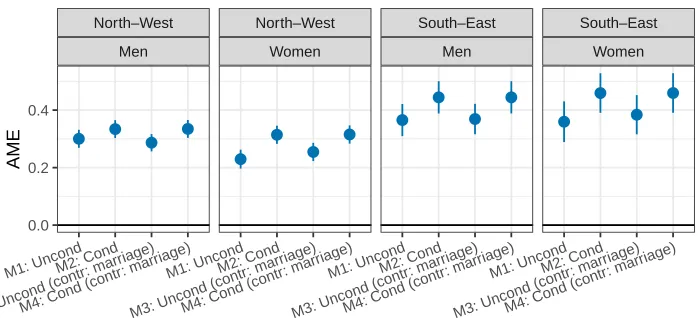
Figure 5 shows AMEs (and 95% confidence intervals) for respondent’s degree in models M1–M4 relative to having no degree. In all cases, the probability of having a child with a degree is higher for respondents with a degree themselves. The tertiary education coefficients are statistically significantly higher in the South and East compared to the North and West.5

5_{Also in M1 and M3, where the confidence intervals overlap for men. Exact results are shown in supplementary}

(14)

Figure 5: Average marginal effects (AMEs) and 95% confidence intervals for respondent’s education in the probability of having a child with tertiary degree (vs. no child or children without degrees) from four types of logit models by region and sex; difference between

respondents with a degree and respondents without. Models M1 and M3 show unconditional estimates, models M2 and M4 conditioning on parenthood. Controlling for year of birth and whether foreign-born in all models, and on marriage in models M3 and M4

North–West

Men

North–West

Women

South–East

Men

South–East

Women

M1: UncondM2: Cond

M3: Uncond (contr

: marriage)

M4: Cond (contr

: marriage)M1: UncondM2: Cond

M3: Uncond (contr

: marriage)

M4: Cond (contr

M3: Uncond (contr

: marriage)

M4: Cond (contr

M3: Uncond (contr

: marriage)

M4: Cond (contr

: marriage) 0.0

0.2 0.4

AME

(15)

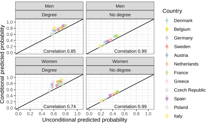
Figure 6: Country-wise unconditional and conditional predicted probabilities of having a child with a degree for average-aged respondents born in the country, separated by sex and education. Countries in Northern and Western Europe are represented with circles and countries in Southern and Eastern Europe with squares. Correlation 0.85 Correlation 0.74 Correlation 0.99 Correlation 0.99 Women Degree Women No degree Men Degree Men No degree

0.0 0.2 0.4 0.6 0.8 1.0 0.0 0.2 0.4 0.6 0.8 1.0 0.0 0.2 0.4 0.6 0.8 1.0 0.0 0.2 0.4 0.6 0.8 1.0

Unconditional predicted probability

Conditional predicted probability

Country Denmark Belgium Germany Sweden Austria Netherlands France Greece Czech Republic Spain Poland Italy

In Figure 6 we revert to the country level to show the relationship between the uncon-ditional and conuncon-ditional estimated probabilities, distinguished by sex and education. The diagonal line shows the point where the probabilities would be equal – but, of necessity, the conditional probabilities must always be greater than or equal to the unconditional and thus they lie on or above the diagonal line. The 95% confidence intervals for the conditional estimates are shown. If the confidence interval does not overlap the diagonal line, the conditional and unconditional estimates are statistically significantly different.

Here we see that (apart from Poland and Czech Republic) the difference between the conditional and unconditional probabilities is larger (and the correlation smaller) for the highly educated. This is because of the educational differentials in the likelihood of having any children (see Figure 2).

(16)

a degree for men and women with no degree in Southern and Eastern Europe (see also Figure 3).

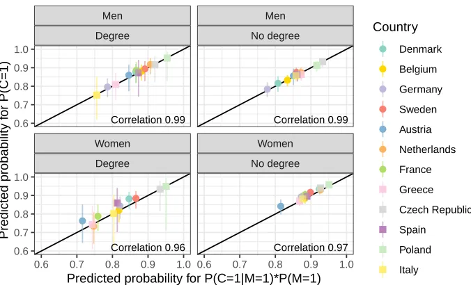
The relationship between the conditional and unconditional probabilities is deter-mined by the probability of having any children. Figure 5 showed that the conditional/un-conditional difference is unaffected by whether or not we took account of marriage. This suggests that the difference is being driven by marital fertility and not by child-bearing among people who never married. This claim is investigated in Figure 7, which shows the country-level results, plotting the predicted probability of having a child against the probability of being married and having a child, distinguishing by sex and education. Again, the diagonal line shows the point where the two predicted probabilities would be the same.

Figure 7: Country-wise predicted probabilities forPPP(((CCC= 1)= 1)= 1)(having a child) andPPP(((CCC= 1= 1= 1|||MMM= 1)= 1)= 1)PPP(((MMM = 1) == 1) == 1) =PPP(((CCC= 1&= 1&= 1&MMM= 1)= 1)= 1) (being married and having a child) for average-aged respondents born in the country, separated by sex and education

Correlation 0.99 Correlation 0.96 Correlation 0.99 Correlation 0.97 Women Degree Women No degree Men Degree Men No degree

0.6 0.7 0.8 0.9 1.0 0.6 0.7 0.8 0.9 1.0

Predicted probability for P(C=1|M=1)*P(M=1)

Predicted probability f

or P(C=1) Country Denmark Belgium Germany Sweden Austria Netherlands France Greece Czech Republic Spain Poland Italy

(17)

The differences between the conditional and unconditional probabilities of having a child with a degree are driven, almost entirely, by whether or not people are married and have children. And the larger conditional/unconditional difference among the higher educated, especially more highly educated women, is due more to educational differences in the likelihood of marriage than to differences in the probability of having a child within marriage.

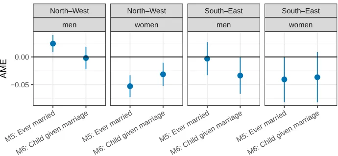
The educational differences in the probability of marriage are shown in Figure 8, which reports average marginal effects for the probability of having ever married (in model M5) and having a child (aged 25 or older) given having ever married (model M6). Women with a degree are less likely to have married in both regions (by 5.3 percentage points in the North and West and 4.1 percentage points in the South and East). Men with a degree in the North–West have a higher probability of marriage (by 2.4 percentage points), whereas in the South–East the difference is small and not statistically significant.

Figure 8: Average marginal effects (AMEs) for respondent’s education in the probability of ever marrying (model M5) and having a child given having ever married (model M6) by region and sex; difference between respondents with a degree (ISCED levels 5–6) and respondents without (ISCED levels 0–4). Controlling for year of birth and whether foreign-born

North–West

men

North–West

women

South–East

men

South–East

women

M5: Ev er marr

ied

M6: Child giv en marr

iage M5: Ev

er marr ied

iage M5: Ev

er marr ied

iage M5: Ev

er marr ied

iage

−0.05 0.00

AME

(18)

difference in probabilities between educational groups is even larger among both women and men (3.4% for men and 3.7% for women), but confidence intervals are wide.

We therefore conclude that, although educational differences play some role in whether married men and women ever have a child, the difference between the conditional and unconditional estimates is mostly driven by educational differences in the likelihood of marriage.

4.1 Spouse’s education

(19)

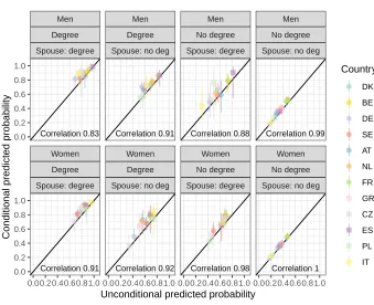
Figure 9: Country-wise unconditional and conditional predicted probabilities of having a child with a degree for ever-married average-aged respondents born in the country, by sex and education of both spouses

Correlation 0.83 Correlation 0.91 Correlation 0.91 Correlation 0.92 Correlation 0.88 Correlation 0.98 Correlation 0.99 Correlation 1 Women Degree Spouse: degree Women Degree Spouse: no deg

Women

No degree Spouse: degree

Women

No degree Spouse: no deg Men

Degree Spouse: degree

Men

Degree Spouse: no deg

Men

No degree Spouse: degree

Men

No degree Spouse: no deg

0.00.20.40.60.81.0 0.00.20.40.60.81.0 0.00.20.40.60.81.0 0.00.20.40.60.81.0 0.0 0.2 0.4 0.6 0.8 1.0 0.0 0.2 0.4 0.6 0.8 1.0

Unconditional predicted probability

Conditional predicted probability

Country DK BE DE SE AT NL FR GR CZ ES PL IT

(20)

Figure 10: Average marginal effects for spouse’s education on the probability of having a child from logit models by respondent’s education, region, and sex; difference between having a spouse with a degree and having a spouse without, controlling for year of birth and whether foreign-born

North–West

men

North–West

women

South–East

men

South–East

women

Degree_{No degree} Degree_{No degree} Degree_{No degree} Degree_{No degree} −0.1

0.0 0.1

AME

Degree

No degree

For women we find no statistically significant differences, although the effect size is large for women in the South and East (8 percentage point increase).

5. Sensitivity analysis

In addition to regional estimates, we have repeated our analyses for each country. The results are shown in Appendix 2. The results confirm that the regional models fit well; the only statistically significant differences are found among Italian women whose estimates are “too high” compared to the regional estimates. Figure A-4 in Appendix 3 shows differences between conditional and unconditional estimates separately for each country. The results show that the differences are more similar between countries in the North and West, while in the South and East there is more variability between countries: In the East (Poland and Czech Republic) the differences are much smaller than in the South (Greece, Spain, and Italy).

(21)

Estimates are also statistically significantly higher for German and Swedish men when compared to the regional model.

Regarding the probability of having children among those who had ever married (Appendix 2.3), the regional model fits fairly well apart from women in Poland, where the estimates are considerably higher and positive rather than negative. In addition, the 95% confidence intervals do not quite overlap the regional estimates in Belgium and for Spanish men (too high) and for German men (too low).

In examining differential fertility, we have only considered people with and with-out children and have not taken into account differences in the number of children that parents might have. In fact, we were unable to do this using SHARE because we do not have data on all siblings; nevertheless, one might wonder whether we would get different results were we able to do so. In fact, we believe that this is probably not the case. While one might argue, for example, that having more children increases the likelihood that at least one will have a degree, the literature on sibship size suggests the opposite: More siblings reduce the educational attainment of children. Lawrence and Breen (2016), in their prospective study using US data and an almost identical design to the one we used, investigated family size effects, and their conclusions about the extent to which educa-tional inequality was reproduced remained unchanged (Lawrence and Breen 2016: 550– 1). Their results showed that the probability of having a child who obtained a college degree did not show a great deal of variation across different family sizes, and the gap in this probability between college-educated and non-college-educated parents was roughly constant at all family sizes.

As a robustness check, we estimated models using the education of a random child instead (Appendix 4). As expected, the results are nearly identical.

6. Discussion

(22)

estimates alike. Despite these differences, the patterns are similar to those reported in earlier research for the United States and Great Britain, though the difference between the conditional and unconditional estimates appears to be rather smaller in these analyses than in those of Lawrence and Breen (2016) and Breen and Ermisch (2017).

The difference between the conditional and unconditional estimates generally in-creased with education, particularly among women. Thus the conditional estimates tend to overstate the extent of educational reproduction. This overstatement is greater for women than men, and the absolute gap between the unconditional and conditional esti-mates is larger in the South and East. Based on Figure 5, and using the results of models M1 and M2, we find that the conditional/unconditional gap for men with and without a degree is 3.4 percentage points in the North and West and 7.9 percentage points in the South and East. For women the comparable figures are 8.5 and 10. When reverting to country-wise estimates (Appendix 2), however, we find a fair amount of variation among the countries, ranging from−0.5 in Denmark to 16.2 in Italy for men and from 2.2 in Czech Republic to 17.9 in Greece for women.

The difference between the conditional and unconditional probabilities depends on the probability of having a child, and this proved to depend entirely on the proportion of people who were married. Childbearing outside marriage plays virtually no role, because rates of marriage were very high and the probability of having a child without ever mar-rying was low in these cohorts. But because very high proportions of married people in our data had at least one child, the crucial thing that gave rise to educational differences in the conditional/unconditional gap was the probability of marriage. More highly edu-cated people, especially women, were less likely to reproduce themselves educationally because they were less likely to marry.

(23)

partner. The selection was based on age and geographical proximity but not on whether they were the respondent’s own or stepchildren.

Regarding spouses, we only used information on the most recent marriage. We did not (mostly, could not) take into account earlier marriages or nonmarital unions, nor whether the most recent spouse was a coparent to any of the respondent’s children or had lived in the same household with them. We did, however, find some evidence that in most cases earlier and current partners had similar education levels. In the rather rare cases of having information on two partners from previously married and currently cohabiting respondents whose current partners also participated in the study (192 respondents, 1.2% of the sample), we found that in 86% of such cases the previous spouse and the current partner had the same education level as measured by having a tertiary degree or not.

Our goal has been, as our title says, to provide a descriptive account. We are not, therefore, making any claims about the causal effect of education on either the probability of having a child or how such a child might fare educationally. We leave these difficult questions to further analyses.

7. Acknowledgments

The authors wish to thank the anonymous reviewers for useful suggestions and comments. The research leading to these results has received funding from the John Fell Oxford University Press (OUP) Research Fund and the Swedish Research Council (DNR 445-2013-7681 and DNR 340-2013-5460).

This paper uses data from SHARE waves 1, 2, 3 (SHARELIFE), 4, and 5 (DOIs: 10.6103/SHARE.w1.500, 10.6103/SHARE.w2.500, 10.6103/SHARE.w3.500,

10.6103/SHARE.w4.500, 10.6103/SHARE.w5.500). See Boersch-Supan et al. (2013) for methodological details.

(24)

References

B¨orsch-Supan, A., Brandt, M., Litwin, H., and Weber, G. (2013). Active ageing and solidarity between generations in Europe. Berlin: De Gruyter.

Breen, R. (2004). Social mobility in Europe. Oxford: Oxford University Press. doi:10.1093/0199258457.001.0001.

Breen, R. and Ermisch, J. (2017). Educational reproduction in Great Britain: A prospec-tive approach.European Sociological Review33(4). doi:10.1093/esr/jcx061.

Erikson, R. and Goldthorpe, J. (1992). The constant flux. A study of class mobility in industrial societies. Oxford: Clarendon Press.

Hillmert, S. (2013). Analysing intergenerational transmissions: From social mobility to social reproduction. Comparative Social Research30: 131–157. doi:10.1108/S0195-6310(2013)0000030009.

Klevmarken, A., Swensson, B., and Hesselius, P. (2005). The SHARE sampling pro-cedures and calibrated design weights. In: B¨orsch-Supan, A. and J¨urges, H. (eds.). The Survey of Health, Ageing and Retirement in Europe – Methodology. Mannheim: Mannheim Research Institute for the Economics of Aging (MEA): 28–69.

Lawrence, M. and Breen, R. (2016). And their children after them? The effect of college on educational reproduction. American Journal of Sociology122(2): 532–572.

Maralani, V. (2013). The demography of social mobility: Black-white differences in the process of educational reproduction. American Journal of Sociology118(6). doi:10.1086/670719.

Mare, R.D. and Maralani, V. (2006). The intergenerational effects of changes in women’s educational attainments. American Sociological Review71(4). doi:10.1177/00031224 0607100402.

OECD (2017).Education at a glance 2017.doi:10.1787/eag-2017-74-en.

Shavit, Y. and Blossfeld, H.P. (1993). Persistent inequalities: A comparative study of educational attainment in thirteen countries. Boulder: Westview Press.

(25)

Appendix

1. Proportion with tertiary education

Table A-1 shows the proportion of tertiary educated in the sample of family respondents born in 1930–1950 in SHARE together with the OECD statistics (OECD 2017). The OECD statistics give the proportion of 55–64-year-olds with tertiary education in 2004 (2003 for Israel). Our sample members were aged 54–74 in 2004, so we would expect the proportions to be similar or lower to those from the OECD statistics. For Israel, Switzerland, and Ireland, both the relative and absolute differences were large.

Table A-1: The proportion of tertiary educated in the sample (unweighted and weighted) and in the OECD statistics for 55–64-year-olds in 2004 (2003 for Israel; OECD, 2017). The last two columns show the ratio and the difference in percentage points between the weighted proportions from the sample and the OECD statistics.

Country Sample (unweighted) Sample (weighted) OECD Ratio Difference

Denmark 33.75 32.93 26.80 1.23 6.13

Belgium 26.33 28.29 20.01 1.41 8.28

Germany 25.76 24.84 22.82 1.09 2.02

Sweden 21.77 21.68 27.26 0.80 −5.58

Austria 20.96 21.57 18.58 1.16 2.99

Netherlands 19.72 19.54 23.97 0.82 −4.43

France 19.13 19.13 14.83 1.29 4.30

Greece 12.18 12.20 11.99 1.02 0.21

Czech Republic 10.41 13.25 10.21 1.30 3.04

Spain 7.40 8.28 12.39 0.67 −4.11

Poland 6.34 6.07 12.24 0.50 −6.17

Italy 5.32 5.44 7.42 0.73 −1.98

Israel 26.81 22.73 43.14 0.53 −20.41

Switzerland 8.31 8.18 22.08 0.37 −13.90

Ireland 38.99 37.34 15.41 2.42 21.93

2. Country-specific models

2.1 Child with degree by respondent’s education

(26)

Figure A-1: Average marginal effects of respondent’s education in the estimated probability of having a child with a tertiary degree (vs. no child or children without degrees) from four types of logit models by country and sex; difference of respondents with a degree to respondents without. Controlling for year of birth and whether foreign-born; also whether ever married in model M2b and M4b. Models M3b and M4b estimated for parents only. Model M4b missing for men in Belgium, Greece, and Poland because there were no never-married fathers in the sample. The dashed lines show estimates from regional models.

ES men ES women PL men PL women IT men IT women

FR men FR women GR men GR women CZ men CZ women

SE men SE women AT men AT women NL men NL women

DK men DK women BE men BE women DE men DE women

M1b: UnondM2b: Cond

M3b: Uncond (contr : marr

iage)

M4b: Cond (contr : marr

iage) M1b: UnondM2b: Cond

iage)

M4b: Cond (contr : marr iage) 0.0 0.2 0.4 0.6 0.8 0.0 0.2 0.4 0.6 0.8 0.0 0.2 0.4 0.6 0.8 0.0 0.2 0.4 0.6 0.8 AME

(27)

2.2 Marriage by respondent’s education

Figure A-2 shows results for the probability of having ever married separately for each country and compares country-wise results to regional results presented in Figure 8.

Figure A-2: Average marginal effects of respondent’s education in the

estimated probability of having ever married from logit models by country and sex; difference between respondents with a degree and respondents without. Controlling for year of birth and whether foreign-born. The dashed lines show estimates from regional models.

France Greece Czech Rep. Spain Poland Italy Denmark Belgium Germany Sweden Austria Netherlands

men women men women men women men women men women men women

−0.2 −0.1 0.0 0.1

AME

P(Ever married)

2.3 Parenthood by respondent’s education

(28)

Figure A-3: The effect of respondent’s education in the estimated probability of having a child given having ever married by country and sex; difference between respondents with a degree and respondents without. Controlling for year of birth and whether foreign-born. The dashed lines show estimates from regional models.

France Greece Czech Rep. Spain Poland Italy Denmark Belgium Germany Sweden Austria Netherlands

men women men women men women men women men women men women

−0.2 −0.1 0.0 0.1

AME

P(Child|Marriage)

3. conditional/unconditional difference by country

(29)

Figure A-4: Differences between unconditional and conditional estimates by country. The dashed lines show estimates from regional models.

men women

DK BE DE SE AT NL FR GR CZ ES PL IT DK BE DE SE AT NL FR GR CZ ES PL IT

0.00 0.05 0.10 0.15

Conditional − Unconditional Diff

erence

Differences between conditional and unconditional estimates

4. Analysis for a random child having degree

(30)

Figure A-5: Comparison of models using any child or a random child. Average marginal effects for respondent’s education in the probability of any/random child having a tertiary degree from four types of logit models by region and sex; difference of respondents with degree to respondents without. Models M1, M1c, M3, and M3c show unconditional estimates, Models M2, M2c, M4, and M4c conditioning on parenthood. Controlling for year of birth and whether foreign-born in all models, and on marriage in Models M3, M3c, M4 and M4c.

South & East

Men

South & East

Women North & West

Men

North & West

Women

M1: Uncond_{M1c: Uncond}M2: CondM2c: Cond

M3: Uncond (contr : marr

iage)

M3c: Uncond (contr : marr

iage)