Variational iteration method for solving nth-order fuzzy integro-differential equations

(1)

Int. J. IndustrialMathematics (ISSN 2008-5621) Vol. 6, No. 3, 2014 Article ID IJIM-00385, 8 pages

Research Article

Variational iteration method for solving

n

th-order fuzzy

integro-differential equations

O. Sedaghatfar ∗ †, S. Moloudzadeh ‡, P. Darabi §

————————————————————————————————–

Abstract

In this paper, the variational iteration method for solvingnth-order fuzzy integro-differential equations (nth-FIDE) is proposed. In fact the problem is changed to the system of ordinary fuzzy integro-differential equations and then fuzzy solution of nth-FIDE is obtained. Some examples show the efficiency of the proposed method.

Keywords: Variational iteration method; nth-order fuzzy integro-differential equations (nth-FIDE); The system of ordinary fuzzy integro-differential equations.

—————————————————————————————————–

1 Introduction

M

ational iteration method (VIM), see [ny authors have been worked about varia-7,8,14,

9] for more details. VIM is an iterative method

which used the Lagrange multipliers. Also several

modifications of VIM can be found in [3, 4, 6].

Because of facility and easy to use, VIM widely employed to various problems. Very recently Ab-basbandy et al. have been considered VIM for

solvingn-th order fuzzy differential equations [2].

In this manuscript, the VIM is extent to solve

nth-FIDE and obtain approximate fuzzy solution.

The VIM is proposed by He [9, 10] as a

modi-fication of a general Lagrange multiplier method

[11]. To illustrate its basic idea of the technique,

we consider following general nonlinear system

L[u(t)] +N[u(t)] =g(t),

∗_{Corresponding author. [email protected]} †_{Department of Mathematics, Shahr-e-rey Branch,} Is-lamic Azad University, shahr-e-rey, Iran.

‡_{Department of Mathematics, Faculty of Science,} Uni-versity of Duhok, Kurdistan Region, Duhok, Iraq.

§_{Department of Mathematics, Borujerd Branch,} Is-lamic Azad University, Borujerd, Iran.

whereLis a linear operator,N is a nonlinear

op-erator, andg(t) is a given construct a correction

functional for the system, which reads

u[k+1](t) =

u[k](t) + ∫ x

a

λ[Lu[k](s) +Nue[k](s)−g(s)]ds,

where λ is a general Lagrange multiplier which

can be identified optimally via variational theory

[9,10,11], the subscriptkdenotes the nth-order

approximation andue[k] _{denotes a restricted}

vari-ation, i.e.,δue[k]= 0.

The structure of this paper is organized as

fol-lows. In Section 2, some basic definitions and

notations which will be used are brought. In

Sec-tion 3, the numerical method to solve nth-FIDE

is proposed. In Section 4, convergency of VIM

for this system is proved. In Section5, the

appli-cation of mentioned method VIM is brought by solving some numerical examples and finally the results are compared with exact solutions.

Con-clusion is drawn in Section6.

(2)

2 Basic Definitions and

Nota-tions

Definition 2.1 An arbitrary fuzzy number is represented by an ordered pair of functions

(u(α), u(α)) for all α ∈ [0,1], which satisfy the following requirements [5]

•u(α)is a bounded left continuous nondecreas-ing function over [0,1];

• u(α) is a bounded left continuous non-increasing function over [0,1];

• u(α)≤u(α), 0≤α ≤1.

Remark 2.1 [1] Let u(α) = (u(α), u(α)), 0 ≤

α≤1 be a fuzzy number, we take

uc(α) = u(α) +u(α)

2 , u

d₍_α_{) =} u(α)−u(α)

2 .

It is clear that ud(α) ≥ 0 and u(α) = uc(α)−

ud(α) and u(α) = uc(α) + ud(α) also a fuzzy numberu∈E is said symmetric ifuc₍_α₎ _is inde-pendent of α for all 0≤α≤1.

Remark 2.2 [1] Let u(α) =

(u(α), u(α)), v(α) = (v(α), v(α)) and also k, s

are arbitrary real numbers. If w=ku+sv then

wc(α) =kuc(α) +svc(α),

wd(α) =|k|ud(α) +|s|vd(α).

Let E be the set of all upper semi-continuous

normal convex fuzzy numbers with bounded α

-level intervals. This means that ifev∈Ethen the

α-level set

[v]α={s|v(s)≥α},

is a closed bounded interval which is denoted by

[v]α = [v(α), v(α)] for α ∈ (0,1], and [v]0 =

∪

α∈(0,1][v]α.

Two fuzzy numbers eu and ev are called equal,

e

u =ev, if u(s) =v(s) for all s∈R or [u]α = [v]α

for all α∈[0,1].

Lemma 2.1 [12] Ifu,e ev∈E, then for α∈(0,1],

[u+v]α= [u(α) +v(α), u(α) +v(α)],

[u.v]α = [minkα,maxkα],

where

kα ={u(α)v(α), u(α)v(α), u(α)v(α), u(α)v(α)}.

Lemma 2.2 [12] Let [v(α), v(α)], α ∈(0,1], be a given family of non-empty intervals. If

(i) [v(α), v(α)]⊃[v(β), v(β)] f or 0< α≤β,

and

(ii) [ lim

k→∞v(αk),klim→∞v(αk)] = [v(α), v(α)],

whenever (αk) is a nondecreasing sequence converging to α ∈ (0,1], then the family

[v(α), v(α)], 0 < α ≤ 1, represent the α-level sets of a fuzzy number v in E. Conversely if

[v(α), v(α)], 0 < α ≤ 1, are the α-level sets of a fuzzy number ev ∈ E, then the conditions (i) and (ii) hold true.

Definition 2.2 [13] Let I be a real interval. A mapping ev : I → E is called a fuzzy pro-cess and we denote the α-level set by [v(t)]α =

[v(t, α), v(t, α)]. The Seikkala derivative ev′(t) of

e

v is defined by

[v′(t)]α= [v ′

(t, α), v′(t, α)],

provided that is a equation defines a fuzzy number

e

v′(t)∈E.

Definition 2.3 [13] The fuzzy integral of fuzzy process ev, ∫_abv(t)dt for a, b∈I, is defined by

[ ∫ b

a

v(t)dt]_α = [ ∫ b

a

v(t, α)dt,

∫ b

a

v(t, α)dt],

provided that the Lebesgue integrals on the right exist.

Definition 2.4 Let ue = (u(α) , u(α)), ve = (v(α), v(α))be fuzzy numbers then the Hausdorff distance between ueand ev is

dH(eu,ev) =

sup_α_∈_[0_,_1]max{|u(α)−v(α)|,|u(α)−v(α)|}.

3 Variational iteration method

In this section, we are going to investigate

solu-tion ofnth-FIDE. Let

                      

e

y(n)(x) =eg(x) +f(x)ye(x) +∫_abk(x, t)ey(m)(t)dt,

e

y(a) =αe0,

e

y′(a) =αe1,

.. . e

y(n−1)(a) =αen−1,

a≤x≤b,

(3)

where αei, i = 0,1, ..., n−1 are fuzzy constant

numbers, m and n are integers and m < n, also

f(x) ≥ 0, k(x, t) are real known functions, and

e

g(x) is fuzzy known function, too. ye(x) is the

solution which to be determined. Using the following assumptions

e

y=ey1, ye

′

=ey2, ye

′′

=ye3, ..., ey(n−1)=eyn,

then equation (3.1) is transformed to the

follow-ing fuzzy integro-differential equations 

                 

e

y₁′ =ye2,

e

y₂′ =ye3,

e

y₃′ =ye4,

.. . e

y_n′ =eg(x) +f(x)ey1(x)

+∫_abk(x, t)eym+1(t)dt,

a≤x≤b,

(3.2) with fuzzy initial conditions

e

y1(a) =αe0, ye2(a) =αe1, ..., yen(a) =αen−1.

Let (g(x;r), g(x;r)) ,(y1(x;r), y1(x;r))

,(y2(x;r), y2(x;r)),...,(yn(x;r), yn(x;r)) for,

0≤r ≤1 and a≤x ≤b are parametric form of

e

g(x),ey1(x),ye2(x), ...,eyn(x), respectively.

Then, parametric form of (3.2) is

                                                  

y′₁ =y₂, y′₂ =y₃, y′₃ =y₄,

.. .

y′_n=g(x) +f(x)y₁(x) +∫_abk(x, t)ym+1(t)dt,

y′₁ =y₂, y′₂ =y₃, y′₃ =y₄,

.. .

y′_n=g(x) +f(x)y₁(x) +∫_abk(x, t)ym+1(t)dt,

(3.3)

where

k(x, t)ym+1(t)

= {

k(x, t)y_m₊₁(t), k(x, t)≥0, k(x, t)y_m₊₁(t), k(x, t)≤0,

k(x, t)ym+1(t)

= {

k(x, t)y_m₊₁(t), k(x, t)≥0, k(x, t)y

m+1(t), k(x, t)≤0.

To solve this system by VIM the following formu-las are obtained:

y[k+1]

j (x) =y

[k]

j (x) +

∫ x

a

λj(x, t)[y ′ j

[k]

(t)

−ey[_jk₊₁] (t)]dt, j= 1,2, ..., n−1,

y[_nk+1](x) =y[_nk](x) + ∫ x

a

λn(x, t)[y ′ n

[k]

(t)

−g(t)−f(t)ey[₁k](t)− ∫ b

a

k(t, s)ey_m[k]₊₁(s)ds]dt,

y[_jk+1](x) =y[_jk](x) + ∫ x

a

λj(x, t)[y ′ j

[k]

(t)

−ey[_jk₊₁] (t)]dt, j= 1,2, ..., n−1,

y[_nk+1](x) =y[_nk](x) + ∫ x

a

λn(x, t)[y ′ n

[k]

(t)

−g(t)−f(t)ey[₁k](t)− ∫ b

a

k(t, s)ey_m[k]₊₁(s)ds]dt,

where λ(x, t) is a general Lagrangian multiplier

which can be identified optimally via variational

theory, ey[k],ey[k]denote a restricted variation, i.e.

δey[k]=δey[k]= 0, andk is iteration step.

The variation is calculated with respect to

y[_jk] (j = 1,2, ..., n), respectively, and δey[k] = 0, then we have

δy[_jk+1](x) =δy[_jk](x) +δ

∫ x

a

λ_j(x, t)[y′_j[k](t)

−ey[_jk₊₁] (t)]dt=δy[_jk](x) +λ_j(x, t)δy_j[k](t)|t=x

− ∫ x

a

∂λ_j(x, t)

dt δy [k]

j (t)dt= (1 +λj(x, x)

δy[_jk](x) + ∫ x

a

(−∂λj(x, t)

dt ) δy [k]

j (t)dt= 0,

j= 1,2, ..., n−1,

δy[_nk+1](x) =δy[_nk](x) +δ

∫ x

a

(4)

−g(t)−f(t)ey[₁k](t)− ∫ b

a

k(t, s)ey_m[k]₊₁(s)ds]dt

=δy[k]

n (x) +λn(x, t)δy

[k]

n (t)|t=x−

∫ x

a

∂λ_n(x, t)

dt

δy[k]

n (t)dt= (1 +λn(x, x)δy

[k]

n (x)

+ ∫ x

a

(−∂λn(x, t)

dt )δy [k]

n (t)dt= 0.

F or j = 1,2, ..., n

−∂λ1(x, t) ∂t =−

∂λ₂(x, t)

∂t =−

∂λ_n(x, t)

∂t = 0,

then

1 +λ_j(x, x) = 0, j= 1,2, ..., n,

and therefor we have

λ_j(x, t) =−1, j= 1,2, ..., n.

Similar to above we have

λj(x, t) =−1, j= 1,2, ..., n,

and we have following iteration formulas                                           

y_j[k+1](x) =y_j[k](x)−∫_ax[y′_j[k](t)−ey[_jk₊₁] (t)]dt, j= 1,2, ..., n−1,

y_n[k+1](x) =y_n[k](x)−∫_ax[y′_n[k](t)−g(t)−f(t) e

y[₁k](t)−∫_abk(t, s)ey[_mk]₊₁(s)ds]dt,

y_j[k+1](x) =y_j[k](x)−∫_ax[y′_j[k](t)−ey[_jk₊₁] (t)]dt, j= 1,2, ..., n−1,

y[nk+1](x) =y[nk](x)−

∫x a[y

′ n

[k]

(t)−g(t)−f(t) e

y[₁k](t)−∫_abk(t, s)ey[_mk]₊₁(s)ds]dt.

(3.4)

4 Convergence Theorem

In this section we analyze the convergency of VIM

for (3.1). Similar to Remark (2.1), let

yc(r) = y(r) +y(r)

2 , y

d₍_r_{) =} y(r)−y(r)

2 ,

then the fuzzy version of (3.1) can be written as

                            

y_j′c(x;r) =yc_j₊₁(x;r), (1≤j≤n−1)

y_n′c(x;r) =gc(x) +f(x)y₁c(x) +∫_abk(x, t)

yc_m₊₁(t)dt,

y_j′d(x;r) =y_jd₊₁(x;r), (1≤j≤n−1)

y_n′d(x;r) =gd(x) +f(x)yd₁(x) +∫_abk(x, t)

yd_m₊₁(t)dt,

(4.5) and

  

y_jc(a;r) = yj(a;r)+yj(a;r)

2 , (1≤j≤n)

y_jd(a;r) = yj(a;r)−yj(a;r)

2 .

Similarly from (3.4) we can obtain the following

formula                                                     

y_j[k+1]c(x, r) =y_j[k]c(x, r)−∫_ax[y_j′[k]c(t, r)

−y[_jk₊₁]c(t, r)]dt, j= 1,2, ..., n−1,

yn[k+1]c(x, r) =yn[k]c(x)−

∫x a[y

′ n

[k]c

(t, r)

−gc(t)−f(t)y₁[k]c(t, r)−∫_abk(t, s)

y_m[k]₊₁c (s, r)ds]dt,

y_j[k+1]d(x, r) =y_j[k]d(x;r)−∫_ax[y′_j[k]d(t, r)

−y[_jk₊₁]d(t, r)]dt, j= 1,2, ..., n−1,

yn[k+1]d(x, r) =yn[k]d(x)−

∫x a[y

′ n

[k]d

(t, r)

−gd(t)−f(t)y₁[k]d(t, r)−∫_abk(t, s)

y[_mk]₊₁d (s, r)ds]dt.

(4.6) Let

e_j[k]c(x, r) =y_j[k]c(x, r)−yc_j(x, r),

obviously             

y_jc(x, r) =y_jc(x, r)−∫_ax[y′_jc(t, r)

−yc_j₊₁(t, r)]dt, j= 1,2, ..., n−1,

y_nc(x, r) =yc_n(x, r)−∫_ax[y′_nc(t, r)−g(t)

−f(t)y₁c(t, r)−∫_abk(t, s)yc_m₊₁(s, r)ds]dt,

then               

e[_jk+1]c(x, r) =e[_jk]c(x, r)−∫_ax[e′_j[k]c(t, r)

−e[_jk₊₁]c(t, r)]dt, j = 1,2, ..., n−1,

e[nk+1]c(x, r) =e[nk]c(x)−

∫x a[e

′ n

[k]c

(t, r)

−f(t)e[₁k]c(t, r)−∫_abk(t, s)e[_mk]₊₁c (s, r)ds]dt.

(5)

The Eqs. (4.7) can be written as follow 

           

e[_jk+1]c(x, r) =∫_axe[_jk₊₁]c(t, r)dt,

j = 1,2, ..., n−1,

e[nk+1]c(x, r) =

∫x a[f(t)e

[k]c

1 (t, r)

+∫_abk(t, s)e_m[k]₊₁c (s, r)ds]dt.

Suppose

|e[_jk]c|= max

a≤t≤b|e

[k]c j (t, r)|,

|e[k]c|= max

j |e

[k]c j |,

j= 1,2, ..., n, k = 0,1, ...,

and

K= max

a≤t,s≤b|k(s, t)|, F = maxa≤t≤x|F(t)|.

Then             

|e[1]_j c(x, r)|≤∫_ax|e_j[0]₊₁c(t, r)|dt≤(x−a)|e[0]c|, j = 1,2, ..., n−1,

e[1]nc(x, r)≤

∫x

a[|f(t)||e

[0]c

1 (t, r)|+

∫b

a|k(t, s)|

|e[0]_m₊₁c (s, r)|ds]dt≤(x−a)|e[0]c|(F+K(b−a)),

also             

|e[2]_j c(x, r)|≤∫_ax|e[1]_j₊₁c(t, r)|dt≤ (x−_2!a)2|e[0]c|, j = 1,2, ..., n−1,

e[2]nc(x, r)≤

∫x

a[|f(t)||e

[1]c

1 (t, r)|+

∫b

a|k(t, s)|

|e[1]_m₊₁c (s, r)|ds]dt≤ (x−_2!a)2|e[0]c|(F+K(b−a))2,

and similarly we can obtain

    

|e[_jk]c(x, r)|≤ (x−_ka_!)k|e[0]c|, j= 1,2, ..., n−1,

e[nk]c(x, r)≤ (x−a)

k

k! |e

[0]c_|₍_F₊_K₍_b₋_a₎₎k_.

Thus     

e[_jk]c(x, r)→0 as k→ ∞, j= 1,2, ..., n−1,

e[nk]c(x, r)→0 as k→ ∞.

(4.8)

In similar way, it can be proven that 

   

e[_jk]d(x, r)→0 as k→ ∞, j = 1,2, ..., n−1,

e[nk]d(x, r)→0 as k→ ∞,

(4.9)

and (4.8), (4.9) imply the convergency of method.

5 Numerical Examples

In this section, four numerical examples are solved by MATLAB for illustration and the ob-tained solutions are compared with the exact so-lutions.

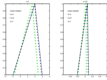
Example 5.1 Consider the following third-order Fuzzy integro-differential equation

                        

e

y′′′(x) =eg(x) +∫₀1(x+t)ye′(t)dt,

e

g= (60x2(r+ 1) +x(1−3r) + (29/3)r

−34/3,−1/6(r−3)(360x2₋₆_x₋₅₎₎_,

e

y(0) = (0,0),

e

y′(0) = (0,0),

e

y′′(0) = (0,0).

(5.10)

The exact solution for this problem is ye(x) =

((r + 1)x5 + (2r −2)x3 , (3−r)x5). See Fig.

1 and Table 1 for comparing the exact solution

and obtained solution by the variational iteration

method for differentk and x.

Example 5.2 Consider the following second-order Fuzzy integro-differential equation

                        

e

y′′(x) =ge(x) +∫₀1(ex+et)ye(t)dt,

e

g= (6(r−1)x+ (1/4−(7/12)r)ex

+ (e−2)r+ 6−2e,1/3(r−2)

(−12 +ex+ 3e)),

e

y(0) = (0,0),

e

y′(0) = (0,0).

(5.11)

The exact solution for this problem is ye(x) =

((r−1)x3+rx2, (2−r)x2). See Fig. 2and Table2

K for comparing the exact solution and obtained solution by the variational iteration method for

(6)

Table 1: numerical result for Example5.1.

dH(ye(k),yeexact)

x k= 5 k= 10 k= 15

0.2 5.8611e-004 1.6689e-005 8.0161e-008

0.4 0.0050 1.4173e-004 6.8076e-007

0.6 0.0178 5.0607e-004 2.4308e-006

0.8 0.0444 0.0013 6.0776e-006

1 0.0913 0.0026 1.2487e-005

dH(ye(k),yeexact)

x k= 10 k= 20 k= 30

0.2 0.0048 3.1510e-004 1.9237e-005

0.4 0.0198 0.0013 8.2562e-005

0.6 0.0457 0.0030 1.8732e-004

0.8 0.0836 0.0054 3.6093e-004

1 0.1346 0.0088 5.6461e-004

                        

e

y′′′(x) =eg(x) +∫₀1(x+t)2ye′(t)dt,

e

g= (−1/15(r+ 1)(15x2−366x+ 10),

1/15(r−3)(15x2−366x+ 10)),

e

y(0) = (0,0),

e

y′(0) = (0,0),

e

y′′(0) = (0,0).

(5.12)

The exact solution of this problem is ey(x) =

((r+ 1)x4 , (3−r)x4). See Fig. 3 and Table

3 for comparing the exact solution and obtained

solution by the variational iteration method for

different kand x.

                        

e

y′′′(x) =eg(x) +∫₀π/2(xcos(t))ey′(t)dt

e

g= (1/2(r−1)(2 sin(x) +x),1/2(1−r)

(2 sin(x) +x))

e

y(0) = (r−1,1−r),

e

y′(0) = (0,0),

e

y′′(0) = (1−r, r−1).

(5.13)

The exact solution of this problem isey(x) = ((r−

1) cos(x) , (1−r) cos(x)). See Fig.4 and Table

4 for comparing the exact solution and obtained

solution by the variational iteration method for

different kand x.

−2 −1 0 1 2 3 4 0

0.1 0.2 0.3 0.4 0.5 0.6 0.7 0.8 0.9 1

−exact solution * k=3 + k=5 . k=7

x=1

−0.4 −0.2 0 0.2 0.4 0.6 0

0.1 0.2 0.3 0.4 0.5 0.6 0.7 0.8 0.9 1

x=1/2

Figure 1: Comparing of exact solution and obtained solution in Example 5.1.

6 Conclusions

In this paper, we used He’s variational iteration

method to obtain fuzzy solution of the nth-order

(7)

un-Table 3: numerical result for Example5.3.

dH(ye(k),yeexact)

x k= 5 k= 10 k= 15

0.2 5.5540e-004 1.9377e-005 1.2624e-007

0.4 0.0050 1.7442e-004 1.1363e-006

0.6 0.0189 6.6002e-004 4.2999e-006

0.8 0.0501 0.0017 1.1385e-005

1 0.1089 0.0038 2.4741e-005

dH(ye(k),yeexact)

x k= 5 k= 10 k= 15

π/8 3.7242e-005 2.9794e-008 8.9369e-011

π/4 5.9587e-004 4.7671e-007 1.4299e-009

3π/4 0.0483 3.8613e-005 1.1582e-007

π/2 0.0095 7.6274e-006 2.2879e-008

−1 −0.5 0 0.5 1 1.5 2 0

0.1 0.2 0.3 0.4 0.5 0.6 0.7 0.8 0.9 1

x=1

−0.20 −0.1 0 0.1 0.2 0.3 0.4 0.5 0.1

0.2 0.3 0.4 0.5 0.6 0.7 0.8 0.9 1

x=1/2

known initial values were constructed. Conver-gency of VIM for this system is proved. The ef-fectiveness of the method was shown by different examples with separable and inseparable kernels.

References

[1] S. Abbasbandy, E. Babolian, M. Alavi,

Nunerical method for solving linear fredholm fuzzy integral equations of the second kind, Chaos, Solitons & Fractals 31 (2007) 138-146.

[2] S. Abbasbandy, T. Allahviranloo, P. Darabi,

O. Sedaghatfar,Variational iteration method

0 1 2 3 4 0

0.1 0.2 0.3 0.4 0.5 0.6 0.7 0.8 0.9 1

x=1

0 0.05 0.1 0.15 0.2 0

0.1 0.2 0.3 0.4 0.5 0.6 0.7 0.8 0.9 1

x=1/2

for solvingn-th order fuzzy differential equa-tions, Math. Comput. Appl., in press.

[3] T. A. Abassy, Modified variational iteration

method (nonlinear homogeneous initial value problem, Comput. Math. Appl. 59 (2010) 912-918.

[4] T. A. Abassy, M. A. El-Tawil, H. El-Zoheiry,

Modified variational iteration method for boussinesq equation, Comput. Math. Appl. 54 (2007) 955-965.

[5] M. Friedman, M. Ming, A. Kandel, Fuzzy

(8)

−1 −0.5 0 0.5 1 0

0.1 0.2 0.3 0.4 0.5 0.6 0.7 0.8 0.9 1

x=1

−1 −0.5 0 0.5 1 0

0.1 0.2 0.3 0.4 0.5 0.6 0.7 0.8 0.9 1

x=1/2

[6] A. Ghorbani, J. Saberi-Nadjafi, An

effec-tive modification of He’s variational iteration method, Nonlinear Anal. Real World Appl. 10 (2009) 2828-2833.

[7] J. H. He,Variational iteration method-a kind

of non-linear analytical technique:Some ex-amples, Int. J. Nonlinear Mech. 34 (1999) 699-708.

[8] J. H. He, Variational iteration method Some

recent result and new interpretations, J. Comput. Appl. Math. 207 (2007) 3-17.

[9] J. H. He, Variational iteration method for delay differential equations, Commun. Non-linear Sci. Numer. Simul. 2 (1997) 235-236.

[10] J. H. He, A new approach to nonlinear

par-tial differenpar-tial equations, Commun. Nonlin-ear Sci. Numer. Simul. 2 (1997) 230-235.

[11] M. Inokuti, H. Sekine, T. Mura,

Gen-eral use of the Lagrange multiplier in non-linear mathematical physics, in: Variational method in the Mechanics of solids, Pergamon press, New York 1978, 156-162.

[12] D. Ralescu,A survey of the representation of

fuzzy concepts and its applications, in: M.M. Gupta, R.K. Ragade, R.R. Yager, Eds., Ad-vances in Fuzzy Set Theory and Applications (North-Holland, Amsterdam (1979) 77-91.

[13] S. Seikkala, On the fuzzy initial value

prob-lem, Fuzzy Sets and Systems 24 (1987)

319-330.

[14] X. Shang, D. Han, Application of the

vari-ational iteration method for solving n th-order integro-differential equations, J. Com-put. Appl. Math. In press.

Omolbanin Sedaghatfar was born in the Tehran, Shahr-e-rey in 1982. She received B.Sc and M.Sc de-gree in applied mathematics from Zahedan Branch, Tehran - Science

and Research Branch, IAU,

re-spectively, and her Ph.D degree in applied mathematics from science and research Branch, IAU, Tehran, Iran in 2011. She is a As-sistant Prof. in the department of mathematics at Islamic Azad University, Shahr-e-rey, Tehran in Iran. She is research interests include numeri-cal solution of fuzzy integro-differential equations and fuzzy differential equation and similar topics.

Saeid Moloudzadeh was born in the Naghadeh-Iran in 1976. He re-ceived B.Sc degree in mathematics and M.Sc degree in applied mathe-matics from Payam-e-Noor Univer-sity of Naghadeh, science and

re-search Branch,IAU to Tehran,

re-spectively, and his Ph.D degree in applied math-ematics from Science and Research Branch, IAU, Tehran, Iran in 2011. He is research interests in-clude fuzzy mathematics, especially, on numerical solution of fuzzy linear systems, fuzzy differential equations and similar topics.

noindent Pejman Darabi was born

in Tehran-Iran in 1978. He

re-ceived B.Sc and M.Sc degrees in applied mathematics from Sabze-var Teacher Education University,

science and research Branch, IAU