Commodity Market and Financial Derivative Instruments: Which Variable Determines the Others?

(1)

Commodity Market and Financial Derivative Instruments: Which Variable Determines the

Others?

M.Leone

1

_{, A. Manelli}

2

_{& R. Pace}

3

Abstract

Over the past decade, agricultural commodity prices underwent wild swings. Periods of high growth in 2008 were followed by periods of sudden decrease in 2009. The excessive increase in food price volatility is a subject of great interest because it has to do with the survival of mankind. Recent academic studies and policy makers have reached sharply different conclusions about the dynamics of such fluctuations. Also, some of them have indicated the main cause in speculative transactions and in the little regulation of futures markets. This paper intends to verify if there exist a co-implication between wheat futures price and some financial „speculative‟ variables. The results of cointegration analysis show that there is no evidence that financial derivative instruments determine the fluctuations of wheat futures price.

Keywords: Financial market, Commodity market, Speculation, GARCH model.

JEL: G10, G15, G23.

1.Introduction

The serious economic crisis which struck many countries worldwide from the Lehman Brothers bankruptcy - showed a rise in prices of agricultural products. In one year - between 2010 and 2011 – in the US market the Wheattkr Spot Index grew by 56,23%, while Gxgrwpsp Forward Index rose by 44,51%.

Price fluctuations can be considered intrinsic in the commodities market because these are linked to the real availability of agricultural raw materials, i.e. the size of supply and demand, as well the variables that affect them such as weather events, climate change and energy prices. However, the excessive increase in price volatility – both rising and decreasing, with sudden fluctuation, even within the same stock market session - has contributed to increasing instability and uncertainty in the agricultural commodity market. The years 2006-2008 and 2010 were periods in which prices rose to worrying levels. This article examines what happens to the prices of real goods – specifically grain – if we assume a different commercial or speculative use of derivatives made from the grain itself as underlying. Notwithstanding, the different purposes that can pursue derivatives: the original, historical, hedging function, used to reduce the overall risk taking position that complement those held on spot markets; and the speculative one, which is aimed, however, at obtaining the maximum profit by taking consistent positions to their expectations about future price trends.

Then, this article investigates the link between spot and futures prices weather financial markets influence the real markets, as stated by journalists and politicians. If it is so, what is the magnitude of such links and how it is achieved. Among academics, Singleton, (2014), sees speculative activity as the determinant of fluctuation in commodity prices.

1_{Università Politecnica delle Marche, PiazzaleMartelli 8, 60121 Ancona (AN), Italy, E-mail: [email protected];}

2_{Università Politecnica delle Marche, PiazzaleMartelli 8, 60121 Ancona (AN), Italy, E-mail:}_{[email protected]}

(2)

The analysis of how speculative activity affects spot markets provides further insights on the role of speculation itself. In particular, analyzing the way that investors are able to change the price and focusing mainly on future prices Brunetti et al., (2015), show the existence of a link - albeit minor - between speculators and volatility, however, emphasizing how investment funds facilitate pricing and reduce market instability. Malliaris and Urrutia, (1996), analyzing the corn future market, find this has a long-term impact on spot prices of corn, wheat and soybeans. Gilbert, (2010), stresses that index investments were the main channel through which monetary and financial activities have influenced food prices in recent years. Especially, he points to the increase in the prices of energy products and metals stimulated interest in agricultural derivatives. This diversification of financial investment was so wide as to determine changes in prices. Usually, when speculation on derivatives is accused to destabilize prices we refer to spot prices: indeed, the futures speculation changes the derivatives prices that, in turn, change the spot market. However, the changes may also result from variation in levels of storage and production. Accordingly, most academics do not fund evidence about possible alteration that speculation would produce on the commodities post market. Indeed, Kim, (2015), suggests that speculators have had a significant and positive influence on the commodity market, during its recent period of financialisation, and, also she believes that restrictions on speculative activity in the futures market are not an efficient way to stabilize the commodity market. In her work, she uses a cross sectional analysis to show the degree of correlation between derivatives speculation and price changes. Furthermore, she analyzes whether the different speculators positions – long or short positions - are one of the causes of such changes. In this regard, she shows that the relationship between price growth and the number of speculative positions is absent or negative. In addition, the correlation value is negative and statistically more significant than smaller increments, when prices rice considerably by adding bigger than 20%, and, finally, the increases do not occur as a result of the speculators purchases. Therefore, Kim finalizes that speculators reduce price growth rather than tighten them up. With regards to the agricultural market, she shows how the hedgers‟ activity have had a greater effect on the prices, rather than the speculators activity. Then, the speculators presence shortens volatility and prevents high real market swings, as well as producing efficiency and liquidity. Ott, (2014), tracks down the main determinant of high volatility in the relationship between closing stock and consumption of food goods – investigating the causes of agricultural price volatility. In this sense, he points out that the speculative activity and the liquidity have had a dampening effect on spot prices in the agricultural derivatives market, whereas, he believes that oil prices and exchange rates are factors that affect volatility. Primarily, the concomitant phenomenon of strong price fluctuations and of growth in index fund4_{activity required an} explanation. According to many observers, the fact that in the agricultural markets the increase in the number of transactions coincided with the sudden rise in prices prove that these transactions push agricultural prices to very high levels and to influence strongly the volatility – i.e. price fluctuations. Consequently, some seek greater regulation of agricultural markets and of electronic markets, as well as the prohibition to make speculative transactions of considerable size. Is there a correlation? Although many observers agree on the causes of the price evolution, the empirical evidence is incomplete and not very conclusive. There is no doubt that in recent years the financial markets activity has increased in agriculture.

However, he concludes that the rise in prices and their volatility are a direct consequence of this evolution is premature.t is true that after 2000, increasingly speculative funds and financial institutions have worked on agricultural exchanges5_{. Critics describe the investment in index funds as excessive speculation.}

4_{The index funds are funds that replicate the movements of specific market indices. They are CIUs, collective investment}

undertakings, seeking absolute positive movements, regardless of the markets in which they invest. The objective of this financial instruments is triple: the purpose of these financial instruments is to optimize the risk-performance ratio, to maintain a low correlation with traditional investment and to obtain positive returns, regardless of market trends through activities unrelated to original investment. The managers use financial derivatives, financial leverage and sophisticated management techniques that generate very high risk, to reduce the overall risk of such diversified portfolio. In the raw materials field, these funds hold a certainly number of differently weighted raw materials. During the purchase or sell of units, it is very important to best represent the index. Generally, fundamentals are ignored. Index funds can exert pressure on agricultural market prices in different ways, often, although, agricultural commodities do not constitute most of these tools. In fact, when raising the price of non-agricultural raw materials, for example oil, the managers need to purchase agricultural products so that the balance between the different units is fair again. This strengthens the link between the different investment categories. In summary, a commodity index fund is a financial asset that invests on different futures or swaps markets with the aim of replicating profits in a price index.

5_{The percentage of wheat contracts traded on the CBOT and held exclusively for speculative purposes is currently about 80%. At}

(3)

This is because long-term fund strategies may affect the balance between supply and demand pushing prices upwards. Furthermore, Masters and white, (2008), show how speculators, such as index funds, following rising price performance, even taking a long position, threaten to intensify further growth. In 2008, according to the Commodity Future Trading Commission the share of index funds on commodity index investments was 24%. The huge and rapid increase of investments in commodity index funds seems to be related to the rising prices in the commodity markets. This correlation is known as „Masters hypothesis‟6_{: he said, earlier, before the US Congress, and then, in front of the} CFTC that speculations on commodity indices strongly influence future prices and distance them from fundamentals. This observation, which is not statistically proven, helped to reinforce the belief that passive speculators have caused a bubble not based on real economic magnitudes in the period of commodity prices volatility.

But assuming an efficient market, the index funds operating in the agricultural market produce a price stabilizing effect, as a direct consequence of their investment strategy. In fact, Index Funds, supporting future prices convergence towards spot prices expected, allow the decrease in the risk premium. As Prehn et al., (2014), even if the Fund pushes the future prices beyond the expected spot prices, the losses will bring some funds out of the market, correcting the imbalance. Particularly, the aforementioned authors argue that hedge funds - having a long-term horizon - stabilize prices both by selling contracts that have increased their value and buying ones that have decreased, and boosting competitive pressure on the same speculators. As the intensified funds work increases liquidity and decreases risk premium, fund activity allows farmers and commercial traders to hedge against price risks on more favorable terms. Moreover, the risk premium reduction, pushing farmers to store part of their crops, mitigates price fluctuations with a positive effect on spot markets too.

Another way in which derivatives markets affect spot prices is through the bond index funds that have futures prices – it is considered an approximation in spot prices. However, to influence commodity prices, the funds should handle physical quantity of goods directly, since their market clearing price is only identified in spot markets where physical goods are bought and sold. Only their supply and demand become relevant to the market price. Indeed, Index Funds invest in futures market trading financial instruments and no physical products. This seems to deny the bubble theory in commodity markets, but some have found some statistical evidence about their effect. Hamilton and Wu, (2015), applying a OLS7_{regression model, from 2006 to 2012, for 12 agricultural commodities,} indicate the absence of index funds on the agricultural products futures. Indeed, to investigate the relationship between the hedge funds activity and the agricultural commodities future prices, they try to predict the weekly profit of a given contract. The model shows that, if „in principle index fund buying of commodity futures could influence pricing of risk‟, they „do not find confirmation of that in the week-to-week variability of the notional value of reported commodity index trader positions‟. Therefore, they don‟t find any relationship between the notional value of commodity futures held by index funds and the expected returns on the market. Although „the increased participation by financial investors in commodity futures markets over the last decade has been quite substantial‟ and potentially able to influence the risk premium, significant changes in the latter.

6_{M.W. Masters, hedge funds manager and Masters Capital Management LLC founder, in May 2008, before the Committee on}

Homeland Security and Governmental Affairs of the United States Senate, said that „Institutional Investor are one of, if not the primary, affecting commodities prices today‟. Starting from the finding that, in recent years, commodity prices have reached very high value, even tripled in five years, suggests that the determinant of such increases is to be identified in Corporate and Government Pension Funds and in other institutional investors that he defines as a whole „Index Speculator‟. These speculators „allocate a portion of their portfolios to investments in the commodity futures market, and behave very differently from the traditional speculators that have always existed in this marketplace‟. Indeed, while the latter provide liquidity by both buying and selling futures, the first „buy futures and then roll their position by buying calendar spreads. They never sell‟. In this way, they consume liquidity and do not provide benefits to the futures markets. Regarding the correlation between their agricultural derivatives market entrance and periods of sudden price increases, Masters specifies that, after the severe equity bear market of 2002, this investors category began to look to the commodity futures market, pouring a liquidity on the main agricultural futures indices, speculating upward. Their strategy has meant that „assets allocated to commodity index trading strategies have risen from $13 billion at the end of 2003 to $260 billion as of March 2008‟, and the prices of the index commodities „have risen by an average of 183% in those five years‟. In Masters‟ opinion, commodity futures prices are the benchmark for the prices of actual physical commodities, so when Index Speculators, with their actions, „drive futures prices higher, the effects are felt immediately in spot prices and in the real economy‟. Therefore, Masters is asking US Congressional intervention to restrict these operations.

7_{The regression model Ordinary Least Squares, aims to minimize the sum of residues, i.e. the difference between the observed}

(4)

To further confirm, the data provided by the CFTC reports show how some operators, in the futures markets, are „pension funds or other managed funds taking a direct position in the futures contracts‟, while „the majority represent positions by swap dealers, who offer their clients an over-the-counter product that mimics some futures-based index‟. The clearest evidence is provided by Tang and Xiong, (2012), in their analysis that the hypothesis that non-energy commodities, included in the S&P GSCI and in the DJ UBSCI index, are more correlated with oil than the commodity off-index. Their basic assumption is that „other participants in commodity markets, such as traditional speculators and commercial hedgers, have a limited capacity to absorb trades by index investors. As a result, the growing presence of index investors can affect commodity prices‟. Particularly, their analysis shows that the average correlation between indexed commodities was indistinguishable from that of the off-index commodity, until the beginning of the new millennium. In 2009, they found a slight increase in correlation for off-index commodity. Instead, for indexed commodities this correlation climbed to very high levels, overcoming 0.5, while in the previous decade stayed at a stable level, below 0.1. They attribute this difference in growth between the two commodities categories, to the effect of investment funds. This means that commodity prices cannot be entirely determined by fundamental information, such as global demand, but, can also result from trading in index funds. Although, the lack of a structural analysis does not allow them to identify the main factors of market shock, they likely consider that the expectation of an increase in hedge funds trading contributed to the peak rate of 2007-2008. Then, although hedge funds weren‟t the causes of price increases, in recent years, they do not exclude their role, while marginal, in relation of these events.

2.Model: integration, cointegration and causality

Although the relationship spot and futures market is well known and studied, the impact that futures prices have on „speculative variables‟ have not been investigated in depth. This paper will fill in this gap. The aim of this paper is answering to three main research questions: i) How do futures prices affect „speculative variables‟?; ii) Is there a relationship between futures prices and speculative variables?; iii) What is its “direction”?To quantify the effect of the increase in commodity prices, the grain in the present case and analyze the trend of those that are defined - during work - as speculative variables, a Co integration analysis is carried out.

This is useful for understanding Forward price developments and other variables that are used, and for establishing the presence and direction of causality. For this purpose, we will examine the following econometric tools:

1. The Cointegration approach of JOHANSEN and JUSELIUS to investigate the existence of the Co integration relationship.

2. The Vector Error Correction Model (VECM) to examine the short and long-term dynamic relationship. 3.The Granger causality test through the VECM to highlight the direction of causality.

1.Johansen

The Johansen test is used to verify the null hypothesis of non-Cointegration between the Forward prices and other speculative variables, against the alternative hypothesis of Cointegration. Johansen shows two statistic:

 The test of likelihood ratio based on the maximum eigenvalue of the stochastic square root.  The test based on the research of the stochastic matrix.

The two statistic are:

λ_trace r = −T ln 1 − λi n

i=r+1

λ_max r, r + 1 = −Tln(1 − λt+i)

where

λ_iis the correlation of least squares n − r, and

Tis the sample size.

The trace checks the null hypothesis of rCointegrating vectors against the alternative hypothesis of

(5)

2.Vector Error Correction Model

Below is a Vector Error Correction Model, VECM. Let Y_t,i= Xi, Mj , where Xi is the Forward price and

M_jis the vector of speculative variables (Open Interest, Non Commercial Long and Commercial Long Positions, Spread, CIT). If Y is cointegrated a VECM is

∆Y_t,i= α_i + γ_iβ_iY_t−1+ Γj,iΔYt−j,i+ εt,i k

j=1

where

αis a constant vector, while the Γmatrix reflects the short-term aspects of the relationship between elements Y_t,i;

β_iis the Cointegration vector, and

Yis the error correction coefficient.

This provides information on the speed of adjustment towards long-term equilibrium. The error correction coefficient is expected to have a negative sign with range −1 < γ < 0.

3.Granger causality test

Through the Granger causality test one tests if the explanatory variables follow the Forward prices, or vice versa. The test is also used to investigate whether two variables have the same direction. The Granger test is explained as follow:

X_t = α_iΔY_t−1+ β_jΔX_t−j+ θ_rECT_t−r + μ_1t

n r=1 n j=1 n i=1

Y_t = λ_i∆X_t−1+ δ_j∆Y_t−j+ ϑ_rECT_t−r+ μ_2t

m r=1 m j=1 m i=1 where

Xtshow the Forward price;

Ytare the speculative variables,

α_i, β_i, λ_i, δ_jare the coefficient;

ECT_t−rrefers to the error correction term derived from long-term correlation;

μ_1,2tare the error terms supposed to be incorrect, and

mandnshow the maximum number of delays.

Do not reject the null hypothesis „X does not Granger-cause Y‟ and reject the null hypothesis „Y does not Granger-cause X‟ means that X changes are Granger-caused by change in Y; namely that lagged Y influences X significantly in the first equation and that lagged X influences Y significantly in the second equation. To verify the existence of a long-run relationship between each two of our variables, the VEC Granger causality test with the MWALD test is implemented. The study uses chi-square statistics to measure causality between the Forward prices and other speculative variables.

3.Data

The chosen variables are:

 the Gxgrwpsp Index8_{, concerning the Future grain prices registered at the Chicago Board of Trade;}  Open Interest that shows the total of all contracts entered into and not yet offset at the date of reference;  Commercial and Non Commercial long positions - we have the first ones if the trader use futures contracts in

that particular commodity for hedging otherwise we have the latter;

 CIT – Commodity Index Trader – long positions, category entered in 2006 by CBOT to indicate speculative indices on commodities, and

 the total Reportable and Non Reportable positions9_.

8_{Source: Bloomberg.}

(6)

The purpose of our analysis is to analyze the trend of wheat prices and that of derivatives positions. For this purpose, data are selected for a 10-year period starting from January 2007 to December 2016.

The table 1 shows the descriptive statistics of the data.

Table 1. Descriptive statistics

It is of particular importance to analyze the last two indicators: skewness and kurtosis. The latter is one of the indices related to the shape of a distribution and is a measure of the „thickness‟ of the tails of a density function, which is the degree of flatness of a distribution. The index corresponding to a normal Gaussian distribution is 3. The value of the variables under consideration are in its surroundings except for Commercial, Non Commercial and CIT positions presenting lower values, therefore we are in the presence of a leptokurtic distribution. The skewness, however, intends to provide a measure of symmetry lack in a distribution. If the distribution is symmetric, the coefficient is zero. The indices of our distribution are all slightly above or below zero. The former – FutUSA, CommL, NReptL e CITL – imply that the mass of the distribution is concentrated on the left. The latter – OpenIn, NCommL and ReptL – imply that the mass of the distribution is concentrated on the right.

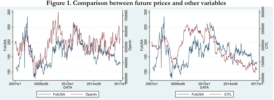
Graphic evidences

(7)

The graphs show that future prices at the beginning of an investigation period - early 2007 - had a reverse trend compared to other „speculative variables‟. After this period, when we hear speculation and prices begin to increase, the two lines follow the same trend accentuating or dampening the fluctuations. However, in 2016 when prices mitigated their volatility they are divided: prices decrease and positions increase. Only exception is for the CIT that - although in early 2007 - show an opposite trend compared to prices.In 2012 they begin to follow the trend accentuating the fluctuations, and continue in the following period until the end of 2016, although dampening the fluctuation, thus diverging from the performance of the other „speculative‟ variables.

4.Findings

The first step of Cointegration analysis is the Augmented Dickey-Fuller Unit Root Test (ADF) to identify the non-stationary condition of variables, i.e. the of a stochastic trend in those individual series. In other words, the ADF test indicates whether the variable has a unit root, or equivalent, that the variable follows a random walk. The null hypothesis is that the variable has a unit root with or without drift so that α is unrestricted and it has also included a trend in the regression. To standardize the variables, we transform them in their natural logarithm. For the study, the ADF test is conducted for all variables considering all possible deterministic components and lag lengths. The test was conducted on all the series and the number of the lagged level terms was chosen based on the SBC information criteria10_.

10_{The Bayesian information criterion or Schwarz criterion is a criterion for selecting a model from a class of parametric models}

with a different number of parameters. The choice of a model to optimize SBC is a form of regularization. When fitting models, it is possible to increase the likelihood by adding parameters, but doing so may result in overfitting. SBC attempt to resolve this problem by introducing a penalty term for the number of parameters in the model. The SBC is formally defined as:

SBC = -2ln(L) + k ln(n)

K=the number of parameters in the stochastic model. N=the number of observations.

(8)

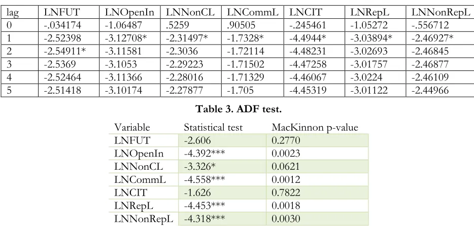
Table 2. SBIC Selection criteria for delays.

lag LNFUT LNOpenIn LNNonCL LNCommL LNCIT LNRepL LNNonRepL

0 -.034174 -1.06487 .5259 .90505 -.245461 -1.05272 -.556712

1 -2.52398 -3.12708* -2.31497* -1.7328* -4.4944* -3.03894* -2.46927* 2 -2.54911* -3.11581 -2.3036 -1.72114 -4.48231 -3.02693 -2.46845 3 -2.5369 -3.1053 -2.29223 -1.71502 -4.47258 -3.01757 -2.46877 4 -2.52464 -3.11366 -2.28016 -1.71329 -4.46067 -3.0224 -2.46109 5 -2.51418 -3.10174 -2.27877 -1.705 -4.45319 -3.01122 -2.44966

Table 3. ADF test.

Variable Statistical test MacKinnon p-value

LNFUT -2.606 0.2770

LNOpenIn -4.392*** 0.0023

LNNonCL -3.326* 0.0621

LNCommL -4.558*** 0.0012

LNCIT -1.626 0.7822

LNRepL -4.453*** 0.0018

LNNonRepL -4.318*** 0.0030

Note: Critical values with trend and intercept are 3.120, -3.410 and -3.960 at the 10%, 5% and 1% level (*, ** and ***, respectively).

From the ADF test we can reject for most of the variables the null hypothesis of unit root at all levels of significance except for the Futures prices and CIT for which the null hypothesis of unit root cannot be rejected. Using a different number of delays we reach the same conclusions. This i.e. we do not say that there is a possible linear combination of a long period. As Engel and Granger demonstrate, if two variables are individually integrated in order one; there is a possibility of a causal relationship in at least one direction and can share common stochastic trends. The idea behind cointegration is that there are common forces that commove the variables over time. The presence of cointegration between variables implies that at least one of them can be utilized to help forecast other variables because a valid causal relationship based on the error-correction model exists. The main cointegration test employed in this investigation is the multivariate test based on the autoregressive representation of Johansen and Juselius.

VECM

To test for cointegration or fit cointegrating VECMs, we must specify how many lags to include. Building on the work of Tsay (1984) and Paulsen (1984), Nielsen (2001) has shown that the methods implemented in the VAR model can be used to determine the lag order. In order to get optimal lag length for cointegration analysis, we have used four criteria:

 Final Prediction Error (FPE);  Akaike Information Criterion (AIC);

 Schwarz Information Criterion or Bayesian (SBIC), and  Hannan-Quinn Information Criterion (HQ).

According to them, the appropriate number of lags should be 2 except for Schwarz who indicates 1.

(9)

At this point we must indicate the number of cointegration equations.

Table 5. Johansen co integration.

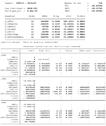
In addition to presenting information to sample size and time intervals, the table shows that the statistics are based on a model with 2 delays and a trend. The central part of the table shows the statistical test and its critical values for the null hypothesis of non cointegration (line 1) and cointegration equations (successive lines). The eigenvalue shown on the last line is used to calculated the statistical trace of the line just above. Johansen‟s testing procedure starts with the test of zero cointegrating equations (a maximum rank of zero) and then accept the first null hypothesis that is not rejected. The model shows there are three cointegration relationships. The results obtained suggest that it is possible to accept the hypothesis that a triple cointegrating vector is present in the model, both for trace and maximum eigenvalue, since the null hypothesis if no cointegration is rejected at three levels of confidence (maximum rank indicates the maximum number of cointegrating vectors). This implies that there exists a significant three cointegrating relationship; consequently, there should be a long-run relationship between Future prices and its determinants.

Dynamic Cointegration

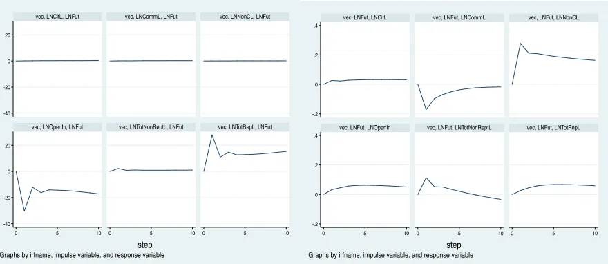
Once verified that variables follow unit-root processes and they are cointegrated, we estimate the Vector Error Correction Model (VECM), and impulse response function analysis, to examine the effects of changes in Future prices on the other variable examined, in order to verify their adjustment mechanism.

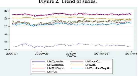
Figure 2. Trend of series.

(10)

The VECM is used to model the stationary relationships between multiple time series containing unit roots.

Table 6. Vector Error Correction Model.

(11)

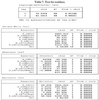
Table 7. Test for residues.

The analysis of estimation and a posteriori analysis of the VECM assume that errors are unrelated.

From the Lagrange-multiplier test we noted that at the level of 5% we cannot reject the null hypothesis that there is no autocorrelation in the residuals for each order (lag) tested. As noted by Johansen Log, likelihood for the VECM is derived by assuming that the errors have a normal distribution and are independently and identically distributed, although many of the asymptotic properties can be derived from the assumption that the errors are merely independent and identically distributed. The Jarque-Bera test is used to analyze skewness and kurtosis after VECM, and to test the null hypothesis that residues are normally distributed. For the individual equations, the null hypothesis is that the disturbance term in that equation has a univariate normal distribution. For all equations jointly, the null hypothesis is that the K disturbances come from a K-dimensional normal distribution. The lack of rejection of the null hypothesis indicates the lack of incorrect specification of the model.

(12)

Figure 3. IRF Graphs.

(13)

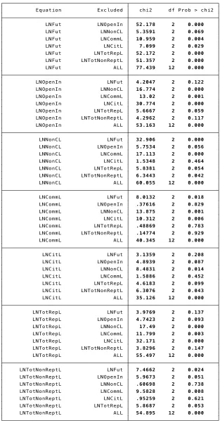
Granger Causality Test

(14)

After the VECM estimation we intend to verify that for each equation and each endogenous variable, which is not the dependent variable in this equation. The coefficient on all delays of an endogenous variable are zero. The null hypothesis is that each endogenous variables do not Granger-cause the dependent variable in this equation. Consider the test results for the first equation. The first is the Wald test to verify that the coefficients LNOpenInt with 2 delays, which appear in the equation for LNFut, are equal to zero. The null hypothesis that LNOpenInt does not Granger-cause LNFut must be rejected. And in the same way for all the other variables. The last line, ALL, is in relation to the null hypothesis that the two delays coefficients of all the other endogenous variables are equal to zero. Since this can be rejected we can reject the null hypothesis that LNOpenIn, LNNonCL, LNCommL, LNCIT, LNRepL and LNNonRepL together do not Granger-cause LNFut.

5.Conclusion

Grain prices from 1960 show a stable growth trend with a few peaks between years ‟70-‟80 and in 2008. Despite a strong decrease, prices are still higher than pre-financial crisis levels and are characterized by high volatility. Several factors help explain market instability. Food safety and the sustainability of food resources are closely linked to political stability11_{. Moreover, agriculture is at the heart of the problems of global population growth, of soil erosion,} of shortage of arable land, of trade financialization.

Then, the search for sustainability indicates that economic growth is possible only within social development, which, in its turn, must be based on respect for and enhancement of the environment. In the achievement of sustainability, the role played by financial and real markets and by their operators, identified in financial, credit or commercial intermediaries, is equally important.

Numerous studies that have put speculation at the base of high food prices have been denied by many academic studies. Climate and country risks are the two main factors behind high prices. At the same time, the confusion about high prices and high volatility – both undesirable – make dynamics even more difficult to interpret. In some developing countries, agricultural prices were pushed up by public authorities to try to make their training more correct.

It is not possible to clearly highlight a direct link between speculation, price growth and market volatility: this is also because the presence of professionals favors a better functioning of the market - incensing liquidity, to the point that the lack of speculation would put the very existence of the market at risk.

Therefore, endogenous and exogenous factors amplify instability. The former are generated by price dynamics; the latter are independent of their fluctuations. Among the former, the dynamics of market fundamentals have a reasonable influence on the price volatility of wheat. For example, stock levels, producer decisions, trade policies – which influence consumptions – imports and exports contribute to determining price dynamics. Among the latter, the connection between the agricultural and energy markets, the dynamics of exchange rates, negative consequences of climate shocks and natural disasters. As volatility is the result of several factors, both endogenous and exogenous, one must evaluate the effects that each of them can generate on international price dynamics.

Futures markets, often blamed for increased volatility, can be an essential element of risk management in physical markets, because they must be able to provide an infrastructure that always guarantees a market price. Jacks, (2007), investigates the relationship between futures markets, speculation and commodity prices volatility and shows that futures markets are systematically associated with lower levels of price volatility.

Despite speculation, commodity trading has been regularly denoted as responsible for high prices and high volatility, especially by governments facing a difficult situation in their country. It is important to keep in mind that in August 2013 the total value of „open interest‟ on agricultural futures was 9.6% of the world production of one year and 3% of the individual annual transactions of all physical markets: therefore, this is a negligible percentage.

11_{States that cannot safe and economic access to food for their populations are much more likely to face protests and suffer}

(15)

Will et al., (2012), analyzing the influential of financial speculation on agricultural commodities, conclude that „according to the current state of research, there is little supporting evidence that the recent increase in financial speculation has caused either a) the price level or b) the price volatility in agricultural markets to rise‟.

6.References

Brunetti C., Buyuksahin B., Harris J.H., 2015, Speculators, prices, and market volatility, in Working Paper, Bank of Canada

Dickey D., Fuller W.A., 1979, Distribution of the estimates for autoregressive time series with unit root, in Journal of the American Statistical Association, Vol. 74, N. 366

Engle R.F., Granger C.W.J., 1987, Co-integration and error correction: representation, estimation, and testing, in Econometrica, Vol. 55, N. 2

Gilbert C.L., 2010, How to understand high food prices, in Journal of Agricultural Economies, Vol. 2, N. 61

Hamilton J.D., Wu J.C., 2015, Effects of index-fund investing on commodities futures prices, in International Economic Review, Vol. 56, N. 1

Jacks D.S., 2007, Populist versus theorist: futures markets and the volatility of prices, in Exploration in Economic History, Vol. 44

Johansen S., Juselius K., 1990, Maximum likelihood estimation and inference on cointegration with applications to the demand for money, in Oxford Bulletin of Economics and Statistics, Vol. 52, N. 2

Kim A., 2015, Does futures speculation destabilize commodity markets?, in Journal of Futures Market, Vol. 35, N. 8 Malliaris A.G., Urrutia J.L., 1996, Linkages between agricultural commodity futures contracts, in Journal of Futures

Market, Vol. 16, N. 5

Masters M.W., 2009, Testimony before the committee on homeland security and government affairs, US Senate Masters M.W., White A.K., 2008, The accidental hunt brothers: how institutional investors are driving up food and

energy prices, Special Report 2008

Nielsen B., 2001, Order determination in general vector autoregressions, in Working Paper, Department of Economics, University of Oxford and Nuffield College

Ott H., 2014, Extent and possible causes of intrayear agricultural commodity price volatility, in Agricultural Economics, Vol. 45

Paulsen J., 1984, Order determination of multivariate autoregressive time series with unit roots, in Journal of Time Series Analysis, Vol. 5, N. 2

Prehn S., Glauben T., Loy J.P, Pie I., Will M.G., 2014, The impact of long-only index funds on price discovery and market performance in agricultural futures market, in Discussion Paper, N. 146, Leibniz Institute of Agricultural Development in Transition Economies

Singleton K.J., 2014, Investor flows and the 2008 boom/bust in oil prices, in Management Science, Vol. 60

Tang K., Xiong W., 2012, Index investment and the financialization of commodities, in Financial Analyst Journal, Vol. 68, N. 6

Tsay R.S., 1984, Order selection in nonstationary autoregressive models, in Annals of Statistics, Vol. 12, N. 4