www.theoryofcomputing.org
Why Simple Hash Functions Work:
Exploiting the Entropy in a Data Stream
Kai-Min Chung
∗Michael Mitzenmacher
†Salil Vadhan
‡Received September 28, 2012; Revised December 17, 2013; Published December 31, 2013
Abstract: Hashing is fundamental to many algorithms and data structures widely used in practice. For the theoretical analysis of hashing, there have been two main approaches. First, one can assume that the hash function is truly random, mapping each data item independently and uniformly to the range. This idealized model is unrealistic because a truly random hash function requires an exponential number of bits (in the length of a data item) to describe. Alternatively, one can provide rigorous bounds on performance when explicit families of hash functions are used, such as 2-universal orO(1)-wise independent families. For such families, performance guarantees are often noticeably weaker than for ideal hashing.
In practice, however, it is commonly observed that simple hash functions, including 2-universal hash functions, perform as predicted by the idealized analysis for truly random
The paper is a merger of the following two conference papers:Why Simple Hash Functions Work: Exploiting the Entropy in a Data Streamby M. M. and S. V.,Proc. 19th Ann. ACM-SIAM Symposium on Discrete Algorithms (SODA), pages 746-755, 2008, andTight Bounds for Hashing Block Sourcesby K-M. C.,Proc. 11th International Workshop, APPROX 2008, and 12th International Workshop, RANDOM 2008, on Approximation, Randomization and Combinatorial Optimization: Algorithms and Techniques, pages 357 - 370, 2008.
∗Work done when visiting U.C. Berkeley, supported by US-Israel BSF grant 2006060 and NSF grant CNS-0430336.
†Supported in part by NSF grants CCF-0915922 and IIS-0964473.
‡Work done in part while visiting U.C. Berkeley. Supported by ONR grant N00014-04-1-0478, NSF grant CCF-0133096,
US-Israel BSF grant 2002246, a Guggenheim Fellowship, and the Miller Institute for Basic Research in Science.
ACM Classification:F.2
AMS Classification:68W20, 68Q25, 68W40
hash functions. In this paper, we try to explain this phenomenon. We demonstrate that the strong performance of universal hash functions in practice can arise naturally from a combination of the randomness of the hash function and the data. Specifically, following the large body of literature on random sources and randomness extraction, we model the data as coming from a “block source,” whereby each new data item has some “entropy” given the previous ones. As long as the Rényi entropy per data item is sufficiently large, it turns out that the performance when choosing a hash function from a 2-universal family is essentially the same as for a truly random hash function. We describe results for several sample applications, including linear probing, chained hashing, balanced allocations, and Bloom filters.
Towards developing our results, we prove tight bounds for hashing block sources, deter-mining the entropy required per block for the distribution of hashed values to be close to uniformly distributed.
1
Introduction
Hashing is at the core of many fundamental algorithms and data structures, including all varieties of hash tables [20], Bloom filters and their many variants [7], summary algorithms for data streams [21], and many others. Traditionally, applications of hashing are analyzed as if the hash function is a truly random function (a. k. a. “random oracle”) mapping each data item independently and uniformly to the range of the hash function. However, this idealized model is unrealistic, because a truly random function mapping {0,1}nto{0,1}mrequires an exponential (inn) number of bits to describe.
For this reason, a line of theoretical work, starting with the seminal paper of Carter and Wegman [8] on universal hashing, has sought to provide rigorous bounds on performance when explicit families of hash functions are used, e. g., ones whose description and computational complexity are polynomial inn
andm. While many beautiful results of this type have been obtained, they are not always as strong as we would like. In some cases, the types of hash functions analyzed can be implemented very efficiently (e. g., universal orO(1)-wise independent hash functions), but the performance guarantees are noticeably weaker than for ideal hashing. (A recent motivating example is the analysis of linear probing under 5-wise independence [25], discussed more below.) In other cases, the performance guarantees are (essentially) optimal, but the hash functions are more complex and expensive (e. g., with a super-linear time or space requirement). For example, if at mostT items are going to be hashed, then aT-wise independent hash function will have precisely the same behavior as an ideal hash function. But aT-wise independent hash function mapping to{0,1}mrequires at leastT·mbits to represent, which is often too large. For some
applications, it has been shown that less independence, such asO(logT)-wise independence, suffices, e. g., [36,26], but such functions are still substantially less efficient than 2-universal hash functions. A series of works [38,24,11] have improved the time complexity of (almost)T-wise independence to a
a significant gap between the theory and practice of hashing.
In this paper, we aim to bridge this gap. Specifically, we suggest that it is due to the use of worst-case analysis. Indeed, in some cases, it can be proven that there exist sequences of data items for which universal hashing does not provide optimal performance. But these bad sequences may be pathological cases that are unlikely to arise in practice. That is, the strong performance of universal hash functions in practice may arise from acombinationof the randomness of the hash function and the randomness of the data.
Of course, doing an average-case analysis, whereby each data item is independently and uniformly distributed in{0,1}n, is also very unrealistic (not to mention that it trivializes many applications). Here
we propose that an intermediate model, previously studied in the literature on randomness extraction [9], may be an appropriate data model for hashing applications. Under the assumption that the data fits this model, we show that relatively weak hash functions achieve essentially the same performance as ideal hash functions.
Our model We model the data as coming from a random source in which the data items can be far from uniform and have arbitrary correlations, provided that each (new) data item is sufficiently unpredictable given the previous items. This is formalized by Chor and Goldreich’s notion of ablock source[9],1where
we require that thei-th item (block)Xihas at least somekbits of “entropy” conditioned on the previous
items (blocks)X1, . . . ,Xi−1. There are various choices for the entropy measure that can be used here;
Chor and Goldreich usemin-entropy, but most of our results hold even for the less stringent measure of
Rényi entropy.
We believe that a block source is a plausible model for many real-life data sources, provided the entropykrequired per-block is not too large. However, in some settings, the data may have structure that violates the block-source property, in which case our results will not apply. Indeed, recent experimental and theoretical results [40,27] have identified some natural classes of data sets (e. g., where the items are densely packed in an interval) where existing universal hash families perform poorly (e. g., when used in linear probing, as described below).
Our work is very much in the same spirit as previous works that have examined intermediate models between worst-case and average-case analysis of algorithms for other kinds of problems. Examples include the semi-random graph model of Blum and Spencer [5], and the smoothed analysis of Spielman and Teng [39]. Interestingly, Blum and Spencer’s semi-random graph models are based on Santha and Vazirani’s model of semi-random sources [35], which in turn were the precursor to the Chor–Goldreich model of block sources [9]. Chor and Goldreich suggest using block sources as an input model for communication complexity, but surprisingly it seems that no one has considered them as an input model for hashing applications.
Our results Our first observation is that standard results in the literature on randomness extractors already imply that universal hashing performs nearly as well ideal hashing, provided the data items have enough entropy [3,17,9,44]. Specifically, if we haveT data items coming from a block source
1Chor and Goldreich called theseprobability-bounded sources,but the termblock sourcehas become more common in the
(X1, . . . ,XT) where each data item has Rényi entropy at least m+2 log(T/ε) and H is a random
2-universal hash function mapping to{0,1}m, then(H(X
1), . . . ,H(XT))has statistical difference at most
ε fromT uniform and independent elements of{0,1}m. Thus, any event that would occur with some probability punder ideal hashing now occurs with probability p±ε. This allows us to automatically translate existing results for ideal hashing into results for universal hashing in our model.
In our remaining results, we focus on reducing the amount of entropy required from the data items. Assuming our hash function has a description sizeo(mT), then we must have at least(1−o(1))mbits of entropy per item for the hashing to “behave like” ideal hashing (because the entropy of(H(X1), . . . ,H(XT))
is at most the sum of the entropies ofHand theXi’s). The standard analysis mentioned above requires an
additional 2 log(T/ε)bits of entropy per block. In the randomness extraction literature, the additional entropy required is typically not significant because log(T/ε)is much smaller thanm. However, it can be significant in our applications. For example, a typical setting is hashingT =Θ(M)items into 2m=M bins. Herem+2 log(T/ε)≥3m−O(1)and thus the standard analysis requires 3 times more entropy than the lower bound of(1−o(1))m. (The bounds obtained for the specific applications mentioned below are even larger, sometimes due to the need for a subconstantε =o(1)and sometimes due to the fact that several independent hash values are needed for each item.)
We use a variety of general techniques to reduce the entropy required. These include switching from statistical difference (equivalently,`1distance) to Rényi entropy (equivalently,`2distance or collision
probability) and/or Hellinger distance (corresponding to`1/2distance under appropriate normalization)
throughout the analysis and decoupling the probability that a hash function is “good” from the uniformity of the hashed valuesh(Xi). In particular, we reduce the required entropy, for(H(X1), . . . ,H(XT))to be
ε-close to uniform in statistical distance, fromm+2 log(T/ε)tom+logT+2 log(1/ε), which we show is tight. We can reduce the entropy required even further for some applications by measuring the quality of the output differently (not using statistical distance) or by using 4-wise independent hash functions (which also have very fast implementations [40]).
Applications We illustrate our approach with several specific applications. Here we informally summa-rize the results; definitions and discussions appear in Sections3and4. In the following discussion,T is the number of data to be hashed,Mis the size of the hash table, and we focus on the typical setting where
T=O(M).
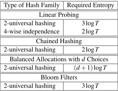
The classic analysis of Knuth [20] gives a tight bound for the insertion time in a hash table withlinear probingin terms of the “load” of the table (the number of items divided by the size of the table), under the assumption that an idealized, truly random hash function is used. Resolving a longstanding open problem, Pagh, Pagh, and Ruži´c [25] recently showed that while pairwise independence does not suffice to bound the insertion time in terms of the load alone (for worst-case data), such a bound is possible with 5-wise independent hashing. However, their bound for 5-wise independent hash functions is polynomially larger than the bound for ideal hashing. We show that 2-universal hashing actually achieves the same asymptotic performance as ideal hashing, provided that the data comes from a block source with roughly 3 logMbits of (Rényi) entropy per item, whereMis the size of the hash table.
Type of Hash Family Required Entropy Linear Probing
2-universal hashing 3 logT
4-wise independence 2 logT
Chained Hashing 2-universal hashing 2 logT
Balanced Allocations withdChoices 2-universal hashing (d+1)logT
Bloom Filters
2-universal hashing 3 logT
Table 1: Each entry denotes the (Rényi) entropy required per item to ensure that the performance of the given application is “close” to the performance when using truly random hash functions. In all cases, the bounds omit additive terms that depend on how close a performance is desired, and we restrict to the (standard) case that the size of the hash table is linear in the number of items being hashed. That is,
m=logT+O(1).
an adversary to choose a set ofT items so that the maximum load is alwaysΩ(T1/2). Our results in turn show that 2-universal hashing achieves the same performance as ideal hashing asymptotically, provided that the data comes from a block source with roughly 2 logT bits of (Rényi) entropy per item.
With thebalanced allocationparadigm [2], it is known that whenT items are hashed toT buckets, with each item being sequentially placed in the least loaded ofd choices (e. g.,d=2), the maximum load is log logT/logd+O(1)with high probability. We show that the same result holds when the hash function is chosen from a 2-universal hash family, provided the data items come from a block source with roughly(d+1)logT bits of entropy per data item.
Bloom filters [4] are data structures for approximately storing sets in which membership tests can result in false positives with some bounded probability. We begin by showing that there is a constant gap in the false positive probability for worst-case data whenO(1)-wise independent hash functions are used instead of truly random hash functions. On the other hand, we show that if the data comes from a block source with roughly 3 logMbits of (Rényi) entropy per item, whereMis the size of the Bloom filter, then the false positive probability with 2-universal hashing asymptotically matches that of ideal hashing.
A summary of required (Rényi) entropy per item for the above applications can be found inTable 1.
2
Preliminaries
Notation [N]denotes the set{1, . . . ,N}. All logs are base 2. For a random variableX and an eventE,
X|E denotesX conditioned onE. ThesupportofXis supp(X) ={x: Pr[X=x]>0}. For a real-valued
function f, E[f(X)],∑xPr[X =x]·f(x)denotes the expectation of f(X), which is also denoted by
Hashing LetHbe a family (multiset) of hash functionsh:[N]→[M]and letHbe uniformly distributed overH. We useh←H to denote thathis sampled according to the distribution H. We say thatH is atruly random familyifHis the set all functions mapping[N]to[M], i. e., theNrandom variables {H(x)}x∈[N] are independent and uniformly distributed over[M]. Fors∈N,H iss-wise independent
(a. k. a.strongly s-universal[42]) if for every sequence of distinct elementsx1, . . . ,xs∈[N], the random
variablesH(x1), . . . ,H(xs)are independent and uniformly distributed over[M]. Hiss-universalif for
every sequence of distinct elementsx1, . . . ,xs∈[N], we have Pr[H(x1) =· · ·=H(xs)]≤1/Ms. The
description size ofH∈H is the number of bits to describe H, which is simply log|H|. For a hash familyHmapping[N]→[M]andk∈N, we defineHk to be the family mapping[N]→[M]kconsisting
of the functions of the formh(x) = (h1(x), . . . ,hk(x)), where eachhi∈H. Observe that ifHiss-wise
independent (resp.,s-universal), then so isHk. However, description size and computation time for functions inHkarektimes larger than forH.
3
Hashing worst-case data
In this section, we describe the four main hashing applications we study in this paper—linear probing, chained hashing, balanced allocations, and Bloom filters—and describe mostly known results about what can be achieved for worst-case data.
3.1 Linear probing
A hash table using linear probing stores a sequencex= (x1, . . . ,xT)of data items from [N]usingM
memory locations. Given a hash functionh:[N]→[M], we place the data itemsx1, . . . ,xT sequentially as
follows. The data itemxifirst attempts placement ath(xi), and if this location is already filled, locations (h(xi) +1)modM,(h(xi) +2)modM, and so on are tried until an empty location is found. The ratio
α=T/M is referred to as theloadof the table. The efficiency of linear probing is measured by the insertion time for a new data item. (Other measures, such as the average time to search for items already in the table, are also often studied, and our results can be generalized to these measures as well.) Definition 3.1. Givenh:[N]→[M], a setx={x1, . . . ,xT−1}of data items from[N]stored via linear
probing usingh, and an extra data itemy∈/x¯, we define theinsertion timeTimeLP(h,x,y)to be the value
of jsuch thatyis placed at locationh(y) + (j−1)modM.
It is well known that with ideal hashing (i. e., hashing using truly random hash functions), the expected insertion time can be bounded quite tightly as a function of the load [20].
Theorem 3.2([20]). Let H be a truly random hash function mapping[N]to[M]. For every sequence x∈[N]T−1and y∈/x, we have
E[TimeLP(H,x,y)]≤1/(1−α)2,
Resolving a longstanding open problem, Pagh, Pagh, and Ruži´c [25] recently showed that the expected lookup time could be bounded in terms ofα using onlyO(1)-wise independence. Specifically, with 5-wise independence, the expected time for an insertion isO 1/(1−α)2.5for any sequencex. On the other hand, in [25] it is also shown that there are examples of sequencesx and pairwise independent hash families such that the expected time for a lookup is logarithmic inT (even though the loadα is independent ofT). In contrast, our work demonstrates that pairwise independent hash functions yield expected lookup times that are asymptotically the same as under the idealized analysis, assuming there is sufficient entropy in the data items themselves.
3.2 Chained hashing
A hash table usingchained hashingstores a setx={x1, . . . ,xT} ∈[N]T in an array ofMbuckets. Leth
be a hash function mapping[N]to[M]. We place each itemxiin the bucketh(xi). Theloadof a bucket
when the process terminates is the number of items in it.
Definition 3.3. Givenh:[N]→[M]and a sequencex={x1, . . . ,xT}of data items from[N]stored via
chained hashing usingh, we define themaximum loadMaxLoadCH(x,h)to be the maximum load among
the buckets after all data items have been placed.
Gonnet [15] proved that whenM=T, the expected maximum load is logT/log logT asymptotically. This bound also holds with high probability, as noted in [28]. More precisely, we have:
Theorem 3.4([15]). Let H be a truly random hash function mapping[N]to[T]. For every sequence x∈[N]T of distinct data items, we have
E[MaxLoadCH(x,H)] = (1+o(1))·
logT
log logT and there is a function g(T) =o(1)such that
Pr
MaxLoadCH(x,H)≤(1+g(T))· logT log logT
=1−o(1),
where the o(1)terms tend to zero as T →∞.
The calculation underlying this theorem requires that the hash function beΩ(logT/log logT)-wise independent. Indeed, Alon et al. [1] demonstrate that this result does not hold in general for 2-universal hash functions. For example, they show that when the hash function is chosen from the (2-universal) family of linear transformationsF2→F for a finite fieldF whose sizeT =|F|is a square, it is possible for an adversary to choose a set ofT items so that the maximum load is always at least√T.
3.3 Balanced allocations
A hash table using the balanced allocation paradigm[2] withd∈Nchoices stores a sequencex=
(x1, . . . ,xT)∈[N]T in an array ofMbuckets. Lethbe a hash function mapping[N]to[M]d∼= [Md], where
we view the components ofh(x)as(h1(x), . . . ,hd(x)). We place the items sequentially by puttingxiin
the least loaded of thedbucketsh1(xi), . . . ,hd(xi)at timei(breaking ties arbitrarily), where theloadof a
Definition 3.5. Givenh:[N]→[M]d, a sequencex= (x1, . . . ,xT)of data items from[N]stored via the
balanced allocation paradigm (withdchoices) usingh, we define themaximum loadMaxLoadBA(x,h)to
be the maximum load among the buckets at timeT+1.
In the case that the number T of items is the same as the number M of buckets and we do bal-anced allocation withd=1 choice (i. e., chained hashing), it is proved [28] that the maximum load is Θ(logT/log logT)with high probability. Remarkably, when the number of choicesd is two or larger, the maximum load drops to be double-logarithmic.
Theorem 3.6([2,41]). For every d≥2andγ>0, there is a constant c such the following holds. Let H
be a truly random hash function mapping[N]to[T]d. For every sequence x∈[N]T of distinct data items, we have
Pr
MaxLoadBA(x,H)>
log logT
logd +c
≤ 1
Tγ.
There are other variations on this scheme, including the asymmetric version due to Vöcking [41] and cuckoo hashing [26]; we choose to study the original setting for simplicity.
The asymmetric scheme has been recently studied under explicit functions [43], similar to those of [11]. At this point, we know of no non-trivial upper or lower bounds for the balanced allocation paradigm using families of hash functions with constant independence, although performance has been tested empirically [6]. Such bounds have been a long-standing open question in this area.
3.4 Bloom filters
ABloom filter[4] represents a setx={x1, . . . ,xT} ⊂[N]using an array ofMbits and`hash functions.
For our purposes, it will be somewhat easier to work with asegmented Bloom filter, where theMbits are partitioned into` disjoint subarrays of sizeM/`, with one subarray for each hash function. We assume thatM/`is an integer. (This splitting does not substantially change the results from the standard approach of having all hash functions map into a single array of sizeM.) As in the previous section, we denote the components of a hash functionh:[N]→[M/`]`∼= [(M/`)`], as providing`hash values
h(x) = (h1(x), . . . ,h`(x))∈[M/`]`in the natural way. The Bloom filter is initialized by setting all bits to 0, and then setting thehi(xj)’th bit to be 1 in thei’th subarray for alli∈[`]and j∈[T]. Given a data
itemy, one tests for membership inxby accepting if thehi(y)’th bit is 1 in thei’th subarray for alli∈[`],
and rejecting otherwise. Clearly, ify∈x, then the algorithm will always accept. However, the algorithm may err ify∈/x.
Definition 3.7. Givenh:[N]→[M/`]`(where`dividesM), a setx={x
1, . . . ,xT}of data items from [N]stored in an`-segment Bloom filter usingh, and an additional data itemy∈[N], we define thefalse positive predicateFalsePosBF(h,x,y)to be 1 ify6∈xand the membership test accepts (i. e., ify∈/xyet
hi(y)∈hi(x)def={hi(xj): j=1, . . . ,T}
for alli=1, . . . , `).
Theorem 3.8([4]). Let H be a truly random hash function mapping[N]to[M/`]`(where`divides M). For every set x∈[N]T of data items and every y∈/x, we have
Pr[FalsePosBF(H,x,y) =1] = 1−
1− `
M
T!`
≈1−e−`T/M`.
In the typical case that M=Θ(T), the asymptotically optimal number of hash functions is`=
(M/T)·ln 2, and the false positive probability is approximately 2−`.
We now turn to the worst-case performance of Bloom filters underO(1)-wise independence. It is folklore that 2-universal hash functions can be used with a constant-factor loss in space efficiency. Indeed, a union bound shows that Pr[hi(y)∈hi(x)]is at mostT·(`/M), compared to 1−(1−`/M)T in the case of
truly random hash functions. This can be generalized tos-wise independent families using the following inclusion-exclusion formula.
Lemma 3.9. Let H:[N]→[M/`]be a hash function chosen at random from a familyH(where`|M). For every sequence x∈[N]T, every y∈/x, and every even s≤T , we have
Pr[H(y)∈H(x)] = T
∑
j=1
(−1)j+1
∑
U⊆T,|U|=jPr[∀k∈U:H(y) =H(xk)]
≤
s−1
∑
j=1
(−1)j+1
∑
U⊆T,|U|=jPr[∀xk∈U:H(y) =H(xk)].
IfHis ans-universal hash family, then the firsts−1 terms of the outer sum above are the same as for a truly random function (namely(−1)j+1· Tj
(`/M)j). This gives the following bound.
Proposition 3.10. Let s be an even constant. Let H be an s-universal family mapping[N]to[M/`] (where`divides M), and let H= (H1, . . . ,H`)be a random hash function fromH`. For every sequence
x∈[N]T of T ≤M/`data items and every y∈/x, we have
Pr[FalsePosBF(H,x,y) =1]≤ 1−
1− `
M T + `T M
s!`
.
Proof. ByLemma 3.9, for eachi=1, . . . , `, we have: Pr[Hi(y)∈Hi(x)]≤ −
s−1
∑
j=1
(−1)j
∑
U⊆T,|U|=jPr[Hi(y) =Hi(xk)∀k∈U]
=−
s−1
∑
j=1 (−1)j·
T j ` M j
(bys-universality)
=− "
1− `
M
T −1−
T
∑
j=s (−1)j·
T j ` M j#
≤1−
1− `
where the last inequality follows by observing that the sum is alternating and thus bounded by
T s
(`/M)2≤(`T/M)s.
Thus,
Pr[FalsePosBF(H,x,y) =1] =Pr[Hi(y)∈Hi(x)∀i]≤ 1−
1− `
M
T
+
`T M
s!`
.
Notice that in the common case that`=Θ(1)and`T ≤M/2 , so that the false positive probability is constant, the above bound differs from the one for ideal hashing by an amount that shrinks rapidly withs. However, whensis constant, the difference remains an additive constant. Another way of interpreting this is that to obtain a given guarantee on the false positive probability usingO(1)-wise independence instead of ideal hashing, one must pay a constant factor in the space for the Bloom filter. The following proposition shows that no better bound can be proved based solely onO(1)-wise independence.
Proposition 3.11. Let s be an even constant. For all N,M, `,T ∈Nsuch that M/`is a prime power and T<min{M/`,N}, there exists an(s+1)-wise independent family of hash functionsHmapping[N]to [M/`]a sequence x∈[N]T of data items, and a y∈[N]\x, such that if H= (H1, . . . ,H`)is a random
hash function fromH`, we have
Pr[FalsePosBF(H,x,y) =1]≥ 1−
1− `
M
T
+Ω
`T M
s!`
.
Proof. Letq=M/`, and letFbe the finite field of sizeq. Associate the elements of[M/`]with elements
ofF, and similarly for the firstM/`elements of[N]. LetH1consist of all polynomials f:F→Fof degree
at mosts; this is an(s+1)-wise independent family. LetH2consist of any(s+1)-wise independent
family mapping[N]\FtoF. For a function f ∈H1 and g∈H2, defineh= f∪g:[N]→[M/`]by h(x) = f(x)ifx∈Fandh(x) =g(x)ifx∈/F. LetHbe the family of all such functions f∪g. We letx
be an arbitrary sequence ofT distinct elements ofF, andyany other element ofF.
Again we compute the false positive probability usingLemma 3.9. The firststerms can be computed exactly as before, using(s+1)-wise independence. For the terms beyonds, we observe that when|U| ≥s, it is the case thathi(y) =hi(xk)for allk∈U if and only ifhi= f∪gfor aconstantpolynomial f. The
Pr[Hi(y)∈Hi(x)] = T
∑
j=1
(−1)j+1
∑
U⊆T,|U|=jPr[∀k∈U:Hi(y) =Hi(xk)]
=
"
s−1
∑
j=1
(−1)j+1· T j ` M j# + " T
∑
j=s
(−1)j+1· T j ` M s# = " 1− 1− `
M
T
+ T
∑
j=s (−1)j·
T j ` M j# + "
s−1
∑
j=0 (−1)j·
T j ` M s# ≥ " 1−
1− `
M T +Ω `T M s# −O
Ts−1·
`
M
s
=1−
1− `
M T +Ω `T M s .
Again, to bound the false positive probability, we simply raise the above to the`-th power.
4
Hashing block sources
4.1 Block sources
We view our data items as being random variables distributed over a finite set of sizeN, which we identify with[N]. We use the following quantities to measure the amount of randomness in a data item. For a random variableX, themax probabilityofX is mp(X) =maxxPr[X=x]. Thecollision probabilityofX
is cp(X) =∑xPr[X=x]2. Measuring these quantities is equivalent to measuring themin-entropy
H∞(X) =min
x log(1/Pr[X=x]) =log(1/mp(X))
and theRényi entropy
H2(X) =log(1/Pr[X=X0]) =log(1/cp(X)),
whereX0 is an i. i. d. copy ofX. IfX is supported on a set of sizeK, then mp(X)≥cp(X)≥1/K(i. e., H∞(X)≤H2(X)≤logK), with equality iffX is uniform on its support. It also holds that mp(X)≤
cp(X)1/2(i. e., H∞(X)≥H2(X)/2), so min-entropy and Rényi entropy are always within a factor of 2 of
each other.
We model a sequence of data items as a sequence(X1, . . . ,XT)of correlated random variables where
each item is guaranteed to have some entropy even conditioned on the previous items.
Definition 4.1(Block Sources). A sequence of random variables(X1, . . . ,XT)taking values in[N]T is a block source with collision probability p per block(respectively,max probability p per block) if for every
i∈[T]and every(x1, . . . ,xi−1)∈supp(X1, . . . ,Xi−1), we have cp(Xi|X1=x1,...,Xi−1=xi−1)≤p(respectively,
Whenmax probabilityis used as the measure of entropy, then this is precisely the model of sources suggested in the randomness extractor literature by Chor and Goldreich [9]. We will mainly use the
collision probabilityformulation as the entropy measure, since it makes our results more general. Definition 4.2. (X1, . . . ,XT)is ablack K-sourceif it is a block source with collision probabilityp=1/K
per block.
The following simple fact relates the collision probability of a joint distribution with its marginal. Lemma 4.3. Let(X,Y)be a joint distribution. We havecp(Y)≤ |supp(X)| ·cp(X,Y).
Proof. It follows by an application of the Cauchy-Schwarz inequality. |supp(X)| ·cp(X,Y) =|supp(X)| ·
∑
x,y
Pr[X =x∧Y =y]2
=
∑
x∈supp(X)
12 !
·
∑
y
Pr[Y=y]2·
∑
x∈supp(X)
Pr[X=x|Y=y]2
!
=
∑
y
Pr[Y =y]2·
∑
x∈supp(X)
Pr[X =x|Y =y]2
!
·
∑
x∈supp(X)
12 !
≥
∑
y
Pr[Y =y]2·
∑
x
Pr[X=x|Y=y]
2
=cp(Y).
Let(X,Y)be jointly distributed random variables. We can define the conditional collision probability ofX conditioning onY as follows.
Definition 4.4. Theconditional collision probabilityofX conditioning onY is cp(X|Y) = E
y←Y[cp(X
|Y=y)].
Theconditional Rényi entropyis H2(X|Y) =log(1/cp(X|Y)).
We note that in general, the chain rule (i. e.,H(X,Y) =H(X) +H(Y |X)) does not hold for Rényi entropy; that is, it is not true in general that cp(X,Y) =cp(X)·cp(Y |X). But this fact is true whenY is uniformly distributed.
Lemma 4.5. Let(X,Y)be jointly distributed random variables such that X is uniformly distributed. We have
cp(X,Y) =cp(X)·cp(Y |X).
Proof. Let(X0,Y0)be an i. i. d. copy of(X,Y). We have
cp(X,Y) =Pr[X=X0∧Y =Y0] =Pr[X=X0]·Pr[Y =Y0|X =X0].
The first term is cp(X)by definition. For the second term, note that whenXis uniformly distributed, the distribution ofX remains uniform after conditioning onX=X0. Thus,
Pr[Y =Y0|X =X0] = E
x←X[Pr[Y=Y
0|
X=X0=x]] = E
x←X[cp(Y
On the other hand, the following lemma says that as in the case of Shannon entropy, conditioning can only decrease the entropy.
Lemma 4.6. Let(X,Y,Z)be jointly distributed random variables. We have
cp(X)≤cp(X|Y)≤cp(X|Y,Z).
Proof. For the first inequality, we have cp(X) =
∑
x
Pr[X =x]2
=
∑
y,y0
Pr[Y=y]·Pr[Y =y0]·
∑
x
Pr[X=x|Y =y]·Pr[X=x|Y =y0]
≤
∑
y,y0
Pr[Y=y]·Pr[Y =y0]·
∑
x
Pr[X=x|Y =y]2
1/2 ·
∑
x
Pr[X=x|Y=y0]2
1/2
= E
y←Y
h
cp(X|Y=y)1/2
i2
≤cp(X |Y).
For the second inequality, observe that for everyyin the support ofY, we have cp(X|Y=y)≤cp((X|Y=y)|(Z|Y=y))
from the first inequality. It follows that cp(X|Y) = E
y←Y[cp(X
|Y=y)]
≤ E
y←Y[cp((X
|Y=y)|(Z|Y=y))]
= E
y←Y[z←(ZE|Y=y)
[cp(X|Y=y,Z=z)] =cp(X|Y,Z).
4.2 Extracting randomness
Arandomness extractor[23] can be viewed as a family of hash functions with the property that for any random variableX with enough entropy, if we pick a random hash functionhfrom the family, thenh(X)
universal hash functions) and minimizing the amount of entropy needed from the sourceX. To do this, we will measure the quality of a hash family in ways that are tailored to our application, and thus we do not necessarily work with the standard definitions of extractors.
In requiring that the hashed valueh(X)be “close” to uniform, the standard definition of an extractor uses the most natural measure of “closeness.” Specifically, for random variablesXandY, taking values in[N], theirstatistical differenceis defined as
∆(X,Y) =max
S⊆[N]
Pr[X∈S]−Pr[Y ∈S].
XandY are calledε-close(resp.,ε-far) if∆(X,Y)≤ε(resp.,∆(X,Y)≥ε).
The classic Leftover Hash Lemma shows that universal hash functions are randomness extractors with respect to statistical difference.
Lemma 4.7(The Leftover Hash Lemma [3,17]). Let H:[N]→[M]be a random hash function from a 2-universal familyH. For every random variable X taking values in[N]withcp(X)≤1/K, we have
cp(H(X)|H)≤1/M+1/K and cp(H,H(X))≤(1/|H|)·(1/M+1/K),
and thus(H,H(X))is(1/2)·p
M/K-close to(H,U[M]).
Notice that the above lemma says that the jointdistribution of (H,H(X))is ε-close to uniform (forε= (1/2)·pM/K); a family of hash functions achieving this property is referred to as a “strong” randomness extractor. Up to some loss in the parameterε (which we will later want to save), this strong extraction property is equivalent to saying that with high probability overh←H, the random variable
h(X)is close to uniform. The above formulation of the Leftover Hash Lemma, passing through collision probability, is attributed to Rackoff [18].
To prove the lemma, let(H0,X0)be an i. i. d. copy of(H,X). We have cp(H(X)|H) = E
h←H[cp(h(X))] =Pr[H(X) =H(X
0
)]
≤Pr[X=X0] +Pr[H(X) =H(X0)|X 6=X0]≤ 1
K+
1
M.
Also, sinceHis uniformly distributed, byLemma 4.5,
cp(H,H(X)) =cp(H)·cp(H(X)|H)≤ 1 |H|·
1
M+
1
K
.
It then relies on the fact that if the collision probability of a random variable is close to that of the uniform distribution, then the random variable is close to uniform in statistical difference. This fact is captured (in a more general form) by the following lemma.
Lemma 4.8. If X takes values in[M]andcp(X)≤1/M+1/K, then: (a) For every function f :[M]→R,
whereµ is the expectation of f(U[M])andσis its standard deviation. In particular, if f takes values
in the interval[a,b], then
|E[f(X)]−µ| ≤ p
(µ−a)·(b−µ)·pM/K.
(b) X is(1/2)·p
M/K-close to U[M].
Proof. By the premise of the lemma,
|E[f(X)]−µ|=
∑
x∈[M]
(f(x)−µ)·(Pr[X=x]−1/M)
≤ s
∑
x∈[M]
(f(x)−µ)2· s
∑
x∈[M]
(Pr[X =x]−1/M)2 (Cauchy-Schwarz)
=
q
M·Var[f(U[M])]·
s
∑
x∈[M]
(Pr[X =x]2−2 Pr[X=x]/M+1/M2)
=√M·σ·pcp(X)−2/M+1/M ≤σ·pM/K.
The “in particular” follows from the fact thatσ[Y]≤p(µ−a)·(b−µ)for every random variableY
taking values in[a,b]and having expectationµ. (Proof:σ[Y]2=E[(Y−a)2]−(µ−a)2≤(b−a)·(µ−
a)−(µ−a)2= (µ−a)·(b−µ).)
Item (b) follows by noting that the statistical difference betweenX andU[M] is the maximum of
|E[f(X)]−E[f(U[M])]|over Boolean functions f, which by Item (a) is at most
p
µ(f)·(1−µ(f))· p
M/K≤(1/2)·pM/K.
While the bound on statistical difference given byLemma 4.8(b) is simpler to state,Lemma 4.8(a) often provides substantially stronger bounds. To see this, suppose there is a bad eventSof vanishing density, i. e.,|S|=o(M), and we would like to say that Pr[X ∈S] =o(1). UsingLemma 4.8(b), we would needK=ω(M), i. e., cp(X) = (1+o(1))/M. But applyingLemma 4.8(a) with f equal to the characteristic function ofS, we get the desired conclusion assuming onlyK =O(M), i. e., cp(X) = O(1/M). Variations ofLemma 4.8(a) can be obtained by using Hölder’s inequality instead of Cauchy-Schwarz in the proof; these variations provide bounds in terms of Rényi entropy of different orders (and different moments of f(U[M])).
The classic approach to extracting randomness from block sources is to simply apply a (strong) randomness extractor, like the one inLemma 4.7, to each block of the source, and uses a union bound over blocks. The bound on the distance from the uniform distribution grows linearly with the number of blocks.
Theorem 4.9 ([9, 44]). Let H:[N]→[M]be a random hash function from a 2-universal family H. For for every block source(X1, . . . ,XT)with collision probability1/K per block, the random variable (H,H(X1), . . . ,H(XT))is(T/2)·
p
Thus, if we have enough entropy per block, universal hash functions behave just like ideal hash functions. How much entropy do we need? To achieve an errorε with the above theorem, we need
K≥MT2/(4ε2). In the next section, we will explore how to improve the quadratic dependence onεand
T.
4.3 Optimized block-source extraction
In this section, we present several optimized variants ofTheorem 4.9. Working with statistical distance, we shave a factor of√T fromTheorem 4.9, which translates to a factor ofT saving in the neededKfor the distribution of hashed value to beε-close to uniform. Recall that a blockK-source(X1, . . . ,XT)is
simply a block source with collision probability 1/Kper block.
Theorem 4.10. Let H :[N]→[M]be a random hash function from a 2-universal familyH. For for every block K-source (X1, . . . ,XT), the random variable (H,H(X1), . . . ,H(XT))is
p
MT/K-close to (H,U[M]T).
Recall thatTheorem 4.9is proven by passing to statistical distance first, and then measuring the growth of distance using statistical distance, which incurs a linear loss in the number of blocksT. As the linear loss in statistical distance is tight in the worst case, we instead measure the growth of distance usingHellinger distance(cf. [14]), and only pass to statistical distance in the end.
In addition to working with the stringent notion of statistical distance, it turns out that for several applications, it suffices to ensure that the hashed value(H(X1), . . . ,H(XT))has (or is statistically close
to having) sufficiently small collision probability, say, within anO(1) factor of that of the uniform distribution. We prove theorems of this form with smaller required entropy from the block source, where Theorem 4.11uses only 2-universal hash functions andTheorem 4.12achieves better bounds using 4-wise independent hash functions.
Theorem 4.11. Let H:[N]→[M]be a random hash function from a 2-universal familyH. For every block K-source(X1, . . . ,XT)and everyε>0, the random variable(H,Y) = (H,H(X1), . . . ,H(XT))is
ε-close to a distribution(H,Z)with collision probability
cp(H,Z)≤ 1 |H| ·MT
1+ M
Kε T
.
In particular, if K≥MT/ε, then(H,Z)has collision probability at most(1+2MT/(εK))/(|H| ·MT). Theorem 4.12. Let H:[N]→[M]be a random hash function from a 4-wise independent familyH. For every block K-source(X1, . . . ,XT)and everyε>0, the random variable(H,Y) = (H,H(X1), . . . ,H(XT)) isε-close to a distribution(H,Z)with collision probability
cp(H,Z)≤ 1
|H| ·MT 1+ M
K +
r 2M K2ε
!T
.
Note that by Lemma 4.3, the conclusions of Theorems 4.11 and 4.12 imply that the collision probability cp(Z)is at most(1+2MT/(εK))/MT and(1+γ)/MT, forγ=2·(MT+p2MT2/ε)/K,
respectively.
We shall prove the above three theorems in the following subsections. As the proof ofTheorem 4.10 is more involved, we prove Theorems4.11and4.12first in Sections 4.3.1and4.3.2, and then prove Theorem 4.10inSection 4.3.3. We further provide several lower bounds inSection 4.4showing that the above theorems are optimal in several aspects.
4.3.1 Small collision probability using 2-universal hash functions
LetH:[N]→[M]be a random hash function from a 2-universal familyH. We first study the conditions under which(H,Y) = (H,H(X1), . . . ,H(XT))isε-close to having collision probabilityO(1/(|H| ·MT)).
This requirement is less stringent than(H,Y)beingε-close to uniform in statistical distance, and so requires less bits of entropy.
The starting point of our analysis is the Leftover Hash Lemma stated inLemma 4.7above, which asserts that if cp(X)≤1/K, then cp(H(X)|H)≤1/M+1/K. Using the Leftover Hash Lemma, we show that for every hashed blockYi, the conditional collision probability cp(Yi|H,Y<i)is at most 1/M+1/K.
Lemma 4.13. Let H :[N]→[M]be a random hash function from a2-universal familyH. Let X = (X1, . . . ,XT)be a block K-source over[N]T. Let(H,Y) = (H,H(X1), . . . ,H(XT)). Thencp(H) =1/|H| and for every i∈[T],cp(Yi|H,Y<i)≤1/M+1/K.
Proof. cp(H) =1/|H|is trivial sinceHis uniformly chosen fromH. Fixi∈[T]. By the definition of blockK-source, for everyx<iin the support ofX<i, cp(Xi|X<i=x<i)≤1/K. By the Leftover Hash Lemma,
we have
cp (Yi|X<i=x<i)|(H|X<i=x<i)
≤1/M+1/K
for everyx<i. It follows that cp(Yi|H,X<i)≤1/M+1/K. Now, noting that the value ofY<iis determined
by that ofH,X<i, we can think of (Yi|H,X<i) asYi first conditioning on (H,Y<i), and then further
conditioning onX<i. ByLemma 4.6, we have
cp(Yi|H,Y<i)≤cp(Yi|H,Y<i,X<i) =cp(Yi|H,X<i)≤1/M+1/K,
as desired.
Lemma 4.13implies that(1/T)·∑icp(Yi|H,Y<i)≤1/M+1/K, which by definition can be rewrite
as
E
(h,y)←(H,Y)
" 1
T T
∑
i=1
cp(Yi|(H,Y<i)=(h,y<i))
# ≤ 1
M+
1
K.
Noting that the collision probability is at least 1/M, Markov’s inequality implies that with probability at least 1−ε over(h,y)←(H,Y),
1
T T
∑
i=1
cp(Yi|(H,Y<i)=(h,y<i))≤
1
M+
1
Kε = 1
M·
1+ M
Kε
. (4.1)
1. First, we show how to fix theε-fraction ofbad (h,y)’s. Namely, we modify at mostε-fraction of the distribution (H,Y) to obtain a distribution(H,Z) = (H,Z1, . . . ,ZT) such that for every (h,z)←(H,Z),
1
T T
∑
i=1
cp(Zi|(H,Z<i)=(h,z<i))≤
1
M·
1+ M
Kε
.
2. Then we show that the above condition is sufficient to imply that cp(H,Z)≤(1/|H| ·MT)·(1+ (M/Kε))T.
We use Lemmas4.14and4.15below to formalize the above two steps.
Lemma 4.14. Let(H,Y) = (H,Y1, . . . ,YT)be jointly distributed random variables overH×[M]T such that with probability at least1−ε over(h,y)←(H,Y), the average conditional collision probability
satisfies
1
T · T
∑
i=1
cp(Yi|(H,Y<i)=(h,y<i))≤
1
M+α.
Then there exists a distribution(H,Z) = (H,Z1, . . . ,ZT)such that(H,Z)isε-close to(H,Y), and for every(h,z)∈supp(H,Z), we have
1
T · T
∑
i=1
cp(Zi|(H,Z<i)=(h,z<i))≤
1
M+α.
Furthermore, the marginal distribution of H is unchanged.
Proof. We define the distribution(H,Z)as follows. • Sample(h,y)←(H,Y).
• If(1/T)·∑Ti=1cp(Yi|(H,Y<i)=(h,y<i))≤1/M+α, then output(h,y).
• Otherwise, let j∈[T]be the least index such that 1
T j
∑
i=1
cp(Yi|(H,Y<i)=(h,y<i))−
1
M
≤αand 1
T j+1
∑
i=1
cp(Yi|(H,Y<i)=(h,y<i))−
1
M
>α.
• Choosewj+1, . . . ,wT←U[M], and output(h,y1, . . . ,yj,wj+1, . . . ,wT).
It is easy to check that (i)(H,Z)is well-defined, (ii)(H,Y)isε-close to(H,Z), (iii) for every(h,z)∈
(H,Z),
1
T · T
∑
i=1
cp(Zi|(H,Z<i)=(h,z<i))≤
1
M+α,
Lemma 4.15. Let X = (X1, . . . ,XT)be a sequence of random variables such that for every x∈supp(X),
1
T T
∑
i=1
cp(Xi|X<i=x<i)≤α.
Then the overall collision probability satisfiescp(X)≤αT.
Proof. By the Arithmetic Mean-Geometric Mean inequality, the inequality in the premise implies
T
∏
i=1
cp(Xi|X<i=x<i)≤α T.
Therefore, it suffices to prove
cp(X)≤ max
x∈supp(X)
T
∏
i=1
cp(Xi|X<i=x<i).
We prove the inequality by induction onT. The base caseT =1 is trivial. Suppose the inequality is true forT−1. We have
cp(X) =
∑
x1Pr[X1=x1]2·cp(X2, . . . ,XT|X1=x1)
≤
∑
x1
Pr[X1=x1]2
! ·max
x1
cp(X2, . . . ,XT|X1=x1)
≤cp(X1)·max x1
max
x2,...,xT T
∏
i=2
cp(Xi|X<i=x<i)
!
=max
x T
∏
i=1
cp(Xi|X<i=x<i),
as desired.
We now finish the proof of Theorem 4.11. By Lemma 4.14, (H,Y)is ε-close to a distribution
(H,Z) = (H,Z1, . . . ,ZT)such that for every(h,z)←(H,Z),
1
T T
∑
i=1
cp(Zi|(H,Z<i)=(h,z<i))≤
1
M·
1+ M
Kε
.
ApplyingLemma 4.15on(Z|H=h)for everyh∈supp(H), we have
cp(H,Z) = 1
|H|·h←EH
cp(Z|H=h)
≤ 1 |H| ·MT ·
1+ M
Kε T
4.3.2 Small collision probability using 4-wise independent hash functions
Here we improve the bound in the previous section using 4-wise independent hash functions. The improvement comes from the fact that when we use 4-wise independent hash functions, we have a concentration result on the conditional collision probability for each block, via the following lemma. Lemma 4.16. Let H :[N]→[M]be a random hash function from a4-wise independent familyH, and X a random variable over[N]withcp(X)≤1/K. Then we have
Var
h←H[cp(h(X))]
≤ 2
MK2.
Proof. Let f(h) =cp(h(X)). We compute the variance Var[f(H)] =E[f(H)2]−E[f(H)]2. LetX0,Y,Y0 be i. i. d. copies ofX. We first recall
E[f(H)] =Pr[H(X) =H(X0)]
=Pr[X=X0] +Pr[X6=X0]·Pr[H(X) =H(X0)|X6=X0] =cp(X) + (1−cp(X))· 1
M,
and note that
E[f(H)2] = E
h←H
[Pr[h(X) =h(X0)]2] =Pr[H(X) =H(X0)∧H(Y) =H(Y0)].
The lemma then follows by the following calculation. Pr[H(X) =H(X0)∧H(Y) =H(Y0)]
≤ Pr[X =X0∧Y =Y0]
+Pr[(X =X0∧Y 6=Y0)∨(X6=X0∧Y=Y0)]
·Pr[H(X) =H(X0)∧H(Y) =H(Y0)|(X=X0∧Y 6=Y0)∨(X=6 X0∧Y =Y0)] +Pr[X6=X0∧Y 6=Y0∧ {X,X0} 6={Y,Y0}]
·Pr[H(X) =H(X0)∧H(Y) =H(Y0)|X6=X0∧Y 6=Y0∧ {X,X0} 6={Y,Y0}] +Pr[{X,X0}={Y,Y0} ∧X6=X0]
·Pr[H(X) =H(X0)∧H(Y) =H(Y0)| {X,X0}={Y,Y0} ∧X 6=X0]
≤ cp(X)2+2cp(X)(1−cp(X))· 1
M+ (1−cp(X)) 2· 1
M2+2cp(X) 2· 1
M
≤ E[f(H)]2+2cp(X) 2
M .
Thus, Var[f(H)]≤2/(MK2).
Lemma 4.17. Let H :[N]→[M]be a random hash function from a 4-wise independent familyH. Let X = (X1, . . . ,XT)be a block K-source over[N]T. Let(H,Y) = (H,H(X1), . . . ,H(XT)). Then with probability at least1−ε over(h,y)←(H,Y),
1
T T
∑
i=1
cp(Yi|(H,Y<i)=(h,y<i))≤
1
M· 1+ M K +
r 2M K2ε
!
.
Theorem 4.12follows immediately by composing Lemmas4.17,4.14, and4.15in the same way as the proof ofTheorem 4.11.
Proof ofLemma 4.17. Recall that we have
E
(h,y)←(H,Y)
" 1
T T
∑
i=1
cp(Yi|(H,Y<i)=(h,y<i))
# ≤ 1
M+
1
K.
Hence, our goal is to upper bound the probability of the value 1
T T
∑
i=1
cp(Yi|(H,Y<i)=(h,y<i))
deviating from its mean byp2/MK2ε. Our strategy is to bound the variance of a properly defined
random variable, and then apply Chebychev’s inequality. ByLemma 4.16, for everyi∈[T], we have Var
h←H
cp(Yi|(H,X<i)=(h,x<i))
≤ 2
MK2, ∀x<i∈supp(X<i). (4.2)
Fixi∈[T], let us try to bound the variance of thei-th block. There are two issues to take care of. First, the variance we have is conditioning onX<iinstead ofY<i. Second, even when conditioning onX<i,
it is possible that the variance is too large:
Var
(h,x)←(H,X)
cp(Yi|(H,X<i)=(h,x<i))
=Ω 1 K2 2
MK2.
The reason is that conditioning on differentX<i=x<i, the collision probability of(Yi|X<i=x<i)may have
different expectations overh←H. Thus, we have to subtract the mean first. Let us define
f(h,x<i) =cp(Yi|(H,X<i)=(h,x<i))− E h←H
cp(Yi|(H,X<i)=(h,x<i))
.
Now, for everyx<i∈supp(X<i), f(H,x<i)has mean 0, and variance≤2/MK2. It follows that
Var
(h,x)←(H,X)
[f(h,x<i)]≤
2
MK2.
We now deal with the issue of conditioning onX<i versusY<i. Let us define g(h,y<i) = E
x<i←(X<i|(H,Y<i)=(h,y<i))
We claim that
cp(Yi|(H,Y<i)=(h,y<i))≤
1
M+
1
K+g(h,y<i).
Indeed, byLemma 4.6and the definition of f andg,
cp(Yi|(H,Y<i)=(h,y<i))≤cp (Yi|(H,Y<i)=(h,y<i))|(Xi|(H,Y<i)=(h,y<i))
= E
x<i←(X<i|(H,Y<i)=(h,y<i))
cp(Yi|(H,X<i)=(h,x<i))
= E
x<i←(X<i|(H,Y<i)=(h,y<i))
f(h,x<i) + E h←H
cp(Yi|(H,X<i)=(h,x<i))
≤g(h,y<i) +
1
M+
1
K.
Also note thatg(H,Y<i)has mean 0 and small variance:
E
(h,y<i)←(H,y<i)
[g(h,y<i)] = E
(h,x)←(H,X)
[f(h,x<i)] =0,
Var
(h,y<i)←(H,y<i)
[g(h,y<i)]≤ Var
(h,x)←(H,X)
[f(h,x<i)]≤
2
MK2.
The above argument holds for every blocki∈[T]. Taking average over blocks, we get
E
(h,y)←(H,Y)
" 1
T T
∑
i=1
g(h,y<i)
#
=0,
Var
(h,y)←(H,Y)
" 1
T T
∑
i=1
g(h,y<i)
# ≤ 2
MK2,
and
1
T T
∑
i=1
cp(Yi|(H,Y<i)=(h,y<i))≤
1 M+ 1 K+ 1 T T
∑
i=1
g(h,y<i)
!
.
Finally, we can apply Chebychev’s inequality to random variable(1/T)·∑ig(H,Y<i)to get the desired
result: with probability 1−ε over(h,y)←(H,Y), 1
T T
∑
i=1
cp(Yi|(H,Y<i)=(h,y<i))≤
1
M· 1+ M
K +
r 2M K2ε
!
.
4.3.3 Statistical distance to uniform distribution
LetH:[N]→[M]be a random hash function form a 2-universal familyH. LetX = (X1, . . . ,XT)be a
As mentioned, the classic result in Theorem 4.9 showed that (H,Y) is (T/2)·p
M/K-close to
(H,U[M]T). The result was proven by passing to statistical distance first, and then measuring the growth of
statistical distance using a hybrid argument, which incurs a linear loss in the number of blocksT. Since without further information, the hybrid argument is tight, to avoid linear loss inT, we have to measure the increase of distance over blocks in another way, and pass to statistical distance only in the end. It turns out that theHellinger distance(cf. [14]) is a good measure for our purposes:
Definition 4.18(Hellinger distance). LetX andY be two random variables over [M]. TheHellinger distancebetweenXandY is
d(X,Y)def= 1
2
∑
i ( pPr[X=i]−pPr[Y =i])
!1/2
=
r 1−
∑
i
p
Pr[X =i]·Pr[Y =i].
Like statistical distance, Hellinger distance is a distance measure for distributions, and it takes value in[0,1]. The following standard lemma says that the two distance measures are closely related. We remark that the lemma is tight in both directions even ifY is the uniform distribution.
Lemma 4.19(cf. [14]). Let X and Y be two random variables over[M]. We have d(X,Y)2≤∆(X,Y)≤
√
2·d(X,Y).
In particular, the lemma allows us to upper-bound the statistical distance by upper-bounding the Hellinger distance. Since our goal is to bound the distance to uniform, it is convenient to work with the following definition.
Definition 4.20(Bhattacharyya Coefficient to Uniform). Let X be a random variable over[M]. The
Bhattacharyya coefficientofX to uniformU[M]is
C(X)def= 1 M
∑
ip
M·Pr[X=i] =1−d(X,U[M])2.
(In general, theBhattacharyya coefficientof random variablesXandY is defined to be 1−d(X,Y)2.) Note thatC(X,Y) =C(X)·C(Y) when X andY are independent random variables, so the Bhat-tacharyya coefficient is well-behaved with respect to products (unlike statistical distance). ByLemma 4.19, if the Bhattacharyya coefficientC(X)is close to 1, thenXis close to uniform in statistical distance. Recall that collision probability behaves similarly. If the collision probability cp(X)is close to 1/M, thenX is close to uniform. In fact, by the following normalization, we can view the collision probability as the 2-norm ofX, and the Bhattacharyya coefficient as the 1/2-norm ofX.
Let f(i) =M·Pr[X=i]fori∈[M]. In terms of f(·), the collision probability is cp(X) = (1/M2)· ∑i f(i)2, andLemma 4.8says that if the “2-norm”M·cp(X) =Ei[f(i)2]≤1+εwhere the expectation is over uniformi∈[M], then∆(X,U)≤
√
ε. Similarly,Lemma 4.19says that if the “1/2-norm”C(X) =
Ei[
p
f(i)]≥1−ε, then∆(X,U)≤ √
ε.
all blocks are independent, then the overall collision probability cp(H,Y)is small, and so(H,Y)is close to uniform. However, this is not true without independence, since 2-norm tends to over-weight heavy elements. In contrast, the 1/2-norm does not suffer this problem. Therefore, our approach is to show that small conditional collision probability implies large Bhattacharyya coefficient. Formally, we have the following lemma.
Lemma 4.21. Let X = (X1, . . . ,XT)be jointly distributed random variables over[M1]× · · · ×[MT]such thatcp(Xi|X<i)≤αi/Mi for every i∈[T]. Then the Bhattacharyya coefficient satisfies
C(X)≥ r
1 α1. . .αT
.
With this lemma, the proof ofTheorem 4.10is immediate.
Proof ofTheorem 4.10. ByLemma 4.13, cp(H) =1/|H|, and cp(Yi|H,Y<i)≤(1+M/K)/Mfor every i∈[T]. ByLemma 4.21, the Bhattacharyya coefficient satisfiesC(H,Y)≥(1+M/K)−T/2≥1−MT/2K
(recall thatK≥MT/ε2). It follows byLemma 4.19that
∆((H,Y),(H,U[M]T))≤
√
2·d((H,Y),(H,U[M]T)) =
√ 2·
q
1−C(H,Y)≤pMT/K≤ε. We proceed to proveLemma 4.21. The main idea is to use Hölder’s inequality to relate two different norms. We recall Hölder’s inequality.
Lemma 4.22(Hölder’s inequality [13]).
• Let F,G be two non-negative functions from[M]toR, and p,q>0satisfying1/p+1/q=1. Let x be a uniformly random index over[M]. We have
E
x[F(x)
·G(x)]≤E
x[F(x) p]1/p·
E
x[G(x) q]1/q.
• In general, let F1, . . . ,Fn be non-negative functions from [M]toR, and p1, . . .pn>0satisfying
1/p1+. . .1/pn=1. We have
E
x[F1(x)· · ·Fn(x)]≤Ex[F1(x)
p1]1/p1· · ·E
x[Fn(x) pn]1/pn.
Towards provingLemma 4.21, we first prove the following lemma that relates the collision probability and the Bhattacharyya coefficient of a random variable, which may be of independent interest. The lemma is in fact a special case ofLemma 4.21withT=1.
Lemma 4.23. Let X be a random variable over [M]with cp(X)≤α/M. Then the Bhattacharyya
coefficient of X satisfies C(X)≥p
1/α.That is, the Hellinger distance satisfies
d(X,U[M])≤
q
Proof. We use Hölder’s inequality to relate the two notions. To do so, we express them using the normalization we mentioned before. Let f(x) =M·Pr[X=x]for everyx∈[M]. In terms of f(·), we want to show that Ex[f(x)2]≤α implies Ex[
p
f(x)]≥p1/α. Note that Ex[f(x)] =1. We now apply
Hölder’s inequality withF= f2/3,G= f1/3, p=3, andq=3/2. We have E
x[f(x)]
≤E
x[f(x) 2]1/3·
E
x[f(x) 1/2]2/3,
which implies
C(X) =E
x[
p
f(x)]≥E
x[f(x)] 3/2/
E
x[f(x)
2]1/2≥p 1/α.
Proof ofLemma 4.21. We prove it by induction onT. The base caseT =1 is exactlyLemma 4.23above. Suppose the lemma is true forT−1, we show that it is true forT. To apply the induction hypothesis, we consider the conditional random variables(X2, . . . ,XT|X1=x)for everyx∈[M1]. For everyx∈[M1]and
j=2, . . . ,T, we define
gj(x) =Mj·cp((Xj|X1=x)|(X2, . . . ,Xj−1|X1=x))
to be the “normalized” conditional collision probability. By the induction hypothesis, we have
C(X2, . . . ,XT|X1=x)≥
p
1/g2(x)· · ·gT(x)
for everyx∈[M1]. Now, let f(x) =M1·Pr[X1=x],and note that by definition, C(X) = E
x←X1
hp
f(x)·C(X2, . . . ,XT|X1=x)
i
.
It follows that
C(X) = E
x←X1
hp
f(x)·C(X2, . . . ,XT|X1=x)
i ≥ E
x←X1
hp
f(x)/g2(x)· · ·gT(x)
i
.
We use Hölder’s inequality twice to show that E
x
hp
f(x)/g2(x)· · ·gT(x)
i
≥p1/α1· · ·αT.
Let us first summarize the constraints we have. By definition, we have Ex[f(x)2]≤α1. Fix j∈ {2, . . . ,T}.
Note that
cp(Xj|X<j) = E x←X1
cp((Xj|X1=x)|(X2, . . . ,Xj−1|X1=x))
= E
x←X1
[gj(x)/Mj] = E x←U[M1]
[f(x)gj(x)]/Mj.
It follows that Ex[f(x)gj(x)]≤αj for j=2, . . . ,T. Now, we apply the second version of Hölder’s
inequality with F1= (f/g2· · ·gT)1/2, Fj = (f gj)1/(T+1) for j=2, . . . ,T, p1 =2/(T+1), and pj =
1/(T+1)for j=2, . . . ,T, which gives
E
x
h
f(x)T/(T+1)i≤E
x
hp
f(x)/g2(x)· · ·gT(x)
i2/(T+1) ·E
x[f(x)g2(x)]
1/(T+1)· · ·
E
x[f(x)gT(x)]
so
E
x
hp
f(x)/g2(x)· · ·gT(x)
i ≥E
x
h
f(x)T/(T+1)i( T+1)/2
·
T
∏
j=2
E
x[
f(x)gj(x)]−1/2
≥E
x
h
f(x)T/(T+1)
i(T+1)/2
·p1/α2· · ·αT.
It remains to lower bound the first term byp1/α1. We apply Hölder again withF = f2/(T+2), G= fT/(T+2),p=T+2, andq= (T+2)/(T+1), which gives
E
x[f(x)]
≤E
x
f(x)21/(T+2) ·E
x
h
f(x)T/(T+1)i(
T+1)/(T+2) ,
so
E
x
h
f(x)T/(T+1)i(T+1)/2≥E
x[f(x)]
(T+2)/2/
E
x
f(x)21/2
≥p1/α1.
Combining the inequalities, we haveC(X)≥p
1/α1· · ·αT.
4.4 Lower bounds
In this section, we provide lower bounds on the entropy needed for the data items. We show that ifK
is not large enough, then for every hash familyH, there exists a blockK-sourceX= (X1, . . . ,XT)such
that the hashed sequenceY = (H(X1), . . . ,H(XT))does not satisfy the desired closeness requirements to
uniform (possibly in conjunction with the hash functionH).
4.4.1 Lower bound for statistical distance to uniform distribution
Let us first consider the requirement for the joint distribution of(H,Y)beingε-close to uniform. When there is only one block, this is exactly the requirement for a “strong extractor.” The lower bound in the extractor literature, due to Radhakrishnan and Ta-Shma [29] shows thatK≥Ω(M/ε2)is necessary, which is tight up to a constant factor. Our goal is to show that when hashingT blocks, the value ofK
required for each block increases by a factor ofT. Intuitively, each block will produce some error (i. e., the hashed value is not close to uniform), and the overall error will accumulate over the blocks, so we need to inject more randomness per block to reduce the error. Indeed, we use this intuition to show that
K≥Ω(MT/ε2)is necessary for the hashed sequence to beε-close to uniform, matching the upper bound inTheorem 4.10. Note that the lower bound holds even for a truly random hash family. Formally, we prove the following theorem.
To prove the theorem, we need to find such anXfor every hash familyH. Following the intuition, we find anXthat incurs a certain error on a single block, and takeX= (X1, . . . ,XT)to beT i. i. d. copies
ofX. More precisely, we first find aK-sourceX such that forΩ(1)-fraction of hash functionsh∈H,
h(X)isΩ(ε/ √
T)-far from uniform. This step is the same as the lower bound proof for extractors [29], which uses the probabilistic method. We pickXto be a randomflat K-source, i. e., a uniform distribution over a random set of sizeK, and show thatX satisfies the desired property with nonzero probability. The next step is to measure how the error accumulates over independent blocks. Note that for a fixed hash functionh, the hashed sequence(h(X1), . . . ,h(XT))consists ofT i. i. d. copies ofh(X). Reyzin [33]
has shown that the statistical distance increases by a factor of√T when we haveT independent copies for smallT. However, Reyzin’s result only shows an increase up to distanceO(δ1/3), whereδ is the statistical distance of the original random variables. We improve Reyzin’s result to show that theΩ(
√
T)
growth continues until the distance reaches some absolute constant. We then use it to show that the joint distribution(H,Y)is far from uniform.
The following lemma corresponds to the first step.
Lemma 4.25. Let N and M be positive integers andε ∈(0,1/4),δ ∈(0,1) real numbers such that N≥M/ε2. Let H:[N]→[M]be a random hash function from an hash familyH. Then there exists an
integer K=Ω(δ2M/ε2), and a flat K-source X over[N], such that with probability at least1−δ over
h←H, h(X)isε-far from uniform.
Proof. LetK=bmin{α·M/ε2,N/2}cfor someα to be determined later. LetX be a random flatK -source over[N]. That is,X=US whereS⊂[N]is a uniformly random sizeKsubset of[N]. We claim
that for every hash functionh:[N]→[M], Pr
S[h(US)isε-far from uniform]≥1−c·
√
α (4.3)
for some absolute constantc. Let us assume (4.3), and prove the lemma first. Since the claim holds for every hash functionh,
Pr
h←H,S[h(US)isε-far from uniform]≥1−c·
√ α.
Thus, there exists a flatK-sourceUSsuch that
Pr
h←H[h(US)isε-far from uniform]≥1−c·
√ α.
The lemma follows by settingα=min{δ2/c2,1/32}. We proceed to prove (4.3). It suffices to show that for everyy∈[M], with probability at least 1−c0·√α over randomUS, the deviation of Pr[h(US) =y]
from 1/Mis at least 4ε/M, wherec0is another absolute constant. That is,
Pr
S
Pr[h(US) =y]−
1
M
≥ 4ε
M
≥1−c0·√α. (4.4)
Again, let us see why (4.4) is sufficient to prove (4.3) first. Let us cally∈[M]isbadforSif
Pr[h(US) =y]−
1
M
≥4ε
Since inequality (4.4) holds for everyy∈[M], we have Pr
S,y[yis bad forS]≥1−c
0·√ α,
whereyis uniformly random over[M]. It follows that Pr
S[at least 1/2-fraction ofyare bad forS]≥1−2c
0·√ α.
Observe that if at least 1/2-fraction ofyare bad forS, then∆(h(X),U[M])≥ε. Inequality (4.3) follows
by settingc=2c0.
It remains to prove (4.4). LetT=h−1(y). We have PrS[h(US) =y] =|S∩T|/|S|. Thus, recall that K≤αM/ε2, (4.4) follows from inequality
Pr
S
|S∩T| −K
M
<4Kε
M
≤c0·
r
Kε2
M ,
which follows by the claim below by settingL=K/M, andβ =4εpK/M. (Working out the parameters, we havec0=4c00,ε<1/4 impliesβ <
√
L, andα≤1/32 impliesβ<1.)
Claim 4.26. Let N,K>1be positive integers such that N>2K, and L∈[0,K/2],β ∈(0,min{1, √
L}) real numbers. Let S⊂[N]be a random subset of size K, and T ⊂[N]be a fixed subset of arbitrary size. We have
Pr
S
h
||S∩T| −L| ≤β √
L
i
≤c00·β,
for some absolute constant c00.
Intuitively, the probability in the claim is maximized when the setT has size NL/K so thatL=
ES[|S∩T|], and the claim follows by observing that in this case, the distribution has deviationΘ(
√
L), and each possible outcome has probabilityO(p1/L). The formal proof of the claim is inAppendix A and is proved by expressing the probability in terms of binomial coefficients, and estimating them using Stirling formula.
The next step is to measure the increase of statistical distance over independent random variables. Lemma 4.27. Let X and Y be random variables over[M]such that∆(X,Y)≥ε. Let X = (X1, . . . ,XT) be T i. i. d. copies of X , and let Y= (Y1, . . . ,YT)be T i. i. d. copies of Y . We have
∆(X,Y)≥min{ε0,c
√
T·ε},
whereε0,c are absolute constants.
Proof. We prove the lemma by the following two claims. The first claim reduces the lemma to the special case thatX is a Bernoulli random variable with biasΩ(ε), andY is a uniform coin. The second claim proves the special case.
For our first claim, we make use of the notion of a randomized function. Recall that with a randomized function, the output f(x)for an inputxis a random variable that may take on different values each time
Claim 4.28. Let X and Y be random variables over[M]such that∆(X,Y) =ε. Then there exists a
randomized function f:[M]→ {0,1}such that f(Y) =U{0,1}, and∆(f(X),f(Y))≥ε/2.
Proof. By the definition, there exists a setT ⊂[M]such that
Pr[X∈T]−Pr[Y ∈T] =ε.
Without loss of generality, we can assume that Pr[Y∈T] =p≤1/2 (because we can take the complement ofT). Letg:[M]→ {0,1}be the indicator function ofT, so we have PrY[g(Y) =1] = p. For every x∈[M], we define f(x) =g(x)∨b, wherebis a biased coin with Pr[b=0] =1/(2(1−p)). The claim follows by observing that
Pr[f(Y) =0] =Pr[g(Y) =0∧b=0] = (1−p)·1/(2(1−p)) =1/2,
and
∆(f(X),f(Y))≥∆(X,Y)·Pr[b=0]≥ε/2.
Claim 4.29. Let X be a Bernoulli random variable over {0,1} such thatPr[X =0] =1/2−ε. Let
X= (X1, . . . ,XT)be T independent copies of X . Then
∆(X,U{0,1}T)≥min{ε0,c
√
Tε},
whereε0,c are absolute constants independent ofε and T .
Proof. Forx∈ {0,1}T, let theweightwt(x)ofxto be the number of 1’s inx. Let S=
x∈ {0,1}T
: wt(x)≤T 2 −
√
T
be the subset of{0,1}T with small weight. (This choice ofSis the main source of improvement in our
proof compared to that of Reyzin [33], who instead considers the set of allxwith weight at mostT/2.) For everyx∈S, we have
Pr[X=x]≤ 1
2T ·(1−ε)
T/2+√T·(
1+ε)T/2− √
T ≤
1−min (√
T·ε 2 ,
1 2
)!
·Pr[U{0,1}T =x].
By standard results on large deviation, we have
Pr[U{0,1}T ∈S]≥Ω(1). Combining the above two inequalities, we get
∆(X,U{0,1}T)≥Pr[U{0,1}T ∈S]−Pr[X ∈S]
≥ 1− 1−min (√
T·ε 2 ,
1 2
)!!
·Pr[U{0,1}T ∈S]
≥min (√
T·ε 2 ,
1 2
) ·Ω(1)
=min{c√Tε,ε0}