ISSN (e): 2250-3021, ISSN (p): 2278-8719 Vol. 04, Issue 04 (April. 2014), ||V1|| PP 01-07
Comparative Study of Bisection, Newton-Raphson and Secant
Methods of Root- Finding Problems
Ehiwario, J.C., Aghamie, S.O.
Department of Mathematics, College of Education, Agbor, Delta State.
Abstract: - The study is aimed at comparing the rate of performance, viz-aviz, the rate of convergence of Bisection method, Newton-Raphson method and the Secant method of root-finding. The software, mathematica 9.0 was used to find the root of the function, f(x)=x-cosx on a close interval [0,1] using the Bisection method, the Newton’s method and the Secant method and the result compared. It was observed that the Bisection method converges at the 52 second iteration while Newton and Secant methods converge to the exact root of 0.739085 with error 0.000000 at the 8th and 6th iteration respectively. It was then concluded that of the three methods considered, Secant method is the most effective scheme. This is in line with the result in our Ref.[4].
Keywords: - Convergence, Roots, Algorithm, Iterations, Bisection method, Newton-Raphson method, Secant method and function
I. INTRODUCTION
Root finding problem is a problem of finding a root of the equation
f
x
0
, wheref
x
is a function of a single variable,x
. Letf
x
be a function, we are interested in findingx
such thatf
0
. The number
is called the root or zero off
x
.f
x
may be algebraic, trigonometric or transcendental function.The root finding problem is one of the most relevant computational problems. It arises in a wide variety of practical applications in Physics, Chemistry, Biosciences, Engineering, etc. As a matter of fact, the determination of any unknown appearing implicitly in scientific or engineering formulas, gives rise to root finding problem [1]. Relevant situations in Physics where such problems are needed to be solved include finding the equilibrium position of an object, potential surface of a field and quantized energy level of confined structure [2]. The common root-finding methods include: Bisection, Newton-Raphson, False position, Secant methods etc. Different methods converge to the root at different rates. That is, some methods are faster in converging to the root than others. The rate of convergence could be linear, quadratic or otherwise. The higher the order, the faster the method converges [3]. The study is at comparing the rate of performance (convergence) of Bisection, Newton-Raphson and Secant as methods of root-finding.
Obviously, Newton-Raphson method may converge faster than any other method but when we compare performance, it is needful to consider both cost and speed of convergence. An algorithm that converges quickly but takes a few seconds per iteration may take more time overall than an algorithm that converges more slowly, but takes only a few milliseconds per iteration [4]. Secant method requires only one function evaluation per iteration, since the value of
f
x
n1 can be stored from the previous iteration [1,4]. Newton’s method, on the other hand, requires one function and the derivative evaluation per iteration. It is often difficult to estimate the cost of evaluating the derivative in general (if it is possible) [1, 4-5]. It seem safe, to assume that in most cases, evaluating the derivative is at least as costly as evaluating the function [4]. Thus, we can estimate that the Newton iteration takes about two functions evaluation per iteration. This disparity in cost means that we can run two iterations of the secant method in the same time it will take to run one iteration of Newton method.In comparing the rate of convergence of Bisection, Newton and Secant methods,[4] used C++programming language to calculate the cube roots of numbers from 1 to 25, using the three methods. They observed that the rate of convergence is in the following order: Bisection method < Newton method < Secant method. They concluded that Newton method is 7.678622465 times better than the Bisection method while Secant method is 1.389482397 times better than the Newton method.
II. METHODS
Given a function
f
x
0
, continuous on a closed interval
a
,
b
, such thatf
a
f
b
0
, then, the function
x
0
f
has at least a root or zero in the interval
a
,
b
. The method calls for a repeated halving of sub-intervals of
a
,
b
containing the root. The root always converges, though very slow in converging [5].Algorithm of Bisection Method for Root- Finding: Inputs: (i)
f
x
– the given function,(ii)
a
0,
b
0 – the two numbers, such thatf
a
f
b
0
.Output: An approximation of the root of
f
x
0
in
a
0,
b
0
, fork
0
,
1
,
2
,...
do until satisfied. Compute
2
k k k
b
a
C
Test if
C
k is the desired root. If so, stop. If
C
kis not the desired root, test iff
C
kf
a
k
0
. If so, setb
k1
C
kanda
k1
C
kOtherwise, set
C
k
b
k1
b
k EndStopping Criteria for Bisection Method
The following are the stopping criteria as suggested by [1]: Let
be the error tolerance, that is we would like to obtain the root with an error of at most of
. Then, acceptx
C
k as a root off
x
0
. If any of the following criteria is satisfied:(i)
f
(
C
k)
(ie the functional value is less than or equal to the tolerance).(ii)
kk k
C
C
C
1(ie the relative change is less than or equal to the tolerance).
(iii)
b
ka
2
)
(
(ie the length of the interval after k iterations is less than or equal to tolerance).
(iv)The number of iterations k is greater than or equal to a predetermined number, say N.
Theorem 1: The number of iterations, N needed in the Bisection method to obtain an accuracy of
is given by:N
2
10 10 10
log
)
(
log
)
(
log
b
oa
oProof: Let the interval length after N iteration be
b
o Na
o2
. So to obtain an accuracy of
b
o
Na
o
2
.That is
( )
2 N bo ao
)
(
2
o o N
a
b
)
log(
2
log
10o o
a
b
N
log
102
log(
)
o o
a
b
N
2
log
)
(
log
10 10
o o
a
b
N
2
log
)
(
log
)
(
log
10 10
10
b
oa
oN
as required.Note: Since the number of iterations, N needed to achieve a certain accuracy depends upon the initial length of the interval containing the root, it is desirable to choose the initial interval
a
0,
b
0
as small as possible.III. NEWTON-RAPHSON METHOD
The Newton-Raphson method finds the slope (tangent line) of the function at the current point and uses the zero of the tangent line as the next reference point. The process is repeated until the root is found [5-7]. The method is probably the most popular technique for solving nonlinear equation because of its quadratic convergence rate. But it is sometimes damped if bad initial guesses are used [8-9].It was suggested however, that Newton’s method should sometimes be started with Picard iteration to improve the initial guess [9]. Newton Raphson method is much more efficient than the Bisection method. However, it requires the calculation of the derivative of a function as the reference point which is not always easy or either the derivative does not exist at all or it cannot be expressed in terms of elementary function [6,7-8]. Furthermore, the tangent line often shoots wildly and might occasionally be trapped in a loop [6]. The function,
f
x
0
can be expanded in theneighbourhood of the root
x
o through the Taylorexpansion:
"
(
(
)
0
!
2
)
(
)
(
)
(
)
(
)
(
2 '
o oo
o
f
x
x
x
x
f
x
x
x
f
x
f
, where x can be seen as a trial valuefor the root at the nth step and the approximate value of the next step
x
k1can be derived from0 ) ( ) ( ) ( )
(xk1 f xk xk1xk f' xk
f .
,...
2
,
1
,
0
,
)
(
'
)
(
1
k
x
f
x
f
x
x
k k kk called the Newton-Raphson method.
Algorithm of the Newton- Raphson Method
Inputs: f(x) –the given function, xo –the initial approximation,
-the error tolerance and N –the maximum number of iteration.Output: An approximation to the root
x
or a message of a failure.Assumption:
x
is a simple root off
x
0
Compute
f
(
x
)
andf
'
(
x
)
Compute
)
(
'
)
(
1 k k k kx
f
x
f
x
x
, for k = 0,1,2,… do until convergence or failure. Test for convergence of failure: If
f
(
x
k)
or
k k kx
x
x
1or k>N, stop.
End.
It was remarked in [1], that if none of the above criteria has been satisfied, within a predetermined, say, N, iteration, then the method has failed after the prescribed number of iteration. In this case, one could try the method again with a different xo. Meanwhile, a judicious choice of xo can sometimes be obtained by drawing the graph of f(x), if possible. However, there does not seems to exist a clear- cut guideline on how to choose a right starting point, xo that guarantees the convergence of the Newton-Raphson method to a desire root.
We implement the function,
f
(
x
)
x
cos
x
0
using the Newton-Raphson method with the aid of the software, Mathematica 9.0.IV. THE SECANT METHOD
As we have noticed, the main setback of the Newton-Raphson method is the requirement of finding the value of the derivative of f(x) at each iterations. There are some functions that are either extremely difficult (if not impossible) or time consuming. The way out out of this, according to [1] is to approximate the derivative by
knowing the values of the function at that and the previous approximation. Knowing
f
(
x
k1)
, we can thenapproximate
f
'
(
x
)
as1 1
)
(
)
(
)
(
'
k k k k kx
x
x
f
x
f
x
f
*Putting * into the Newton iterations, we have:
)
(
)
(
)
)(
(
1 1 1
k k k k k k kx
f
x
f
x
x
x
f
x
x
**Algorithm of Secant Method Input:
f
(
x
)
-the given function,
x
0,
x
1 –the two initial approximation of the root,
-the error tolerance and N –the maximum number of iterations.Output: An approximation of the exact solution
or a message of failure, for k= 1,2,… do until convergence or otherwise. Compute
f
(
x
k)
andf
(
x
k1)
Compute the next approximation
)
(
)
(
)
)(
(
1 1 1
k k k k k k kx
f
x
f
x
x
x
f
x
x
Test for convergence or maximum number of iterations: If
x
k1
x
k
or k>N, stop.We implement the function
f
(
x
)
x
cos
x
0
, using the Secant method with the aid of software, Mathematica 9.0.Analysis of Convergence Rates of Bisection, Newton-Raphson and Secant methods.
Definition: Suppose that the sequence
x
k converges to
. Then, the sequence
x
k is said to converge to
with order of convergence
if there exists a positive constant p such that:
k kx
x
k
1lim
=p
e
e
k k
1lim
.Thus, if
=1, the convergence is linear. If
=2, the convergence is quadratic, and so on. The number
is called the convergence factor. Based on this definition, we show the rate of convergence of Newton and Secant methods of root-finding. Meanwhile, we may not border to show that of Bisection method, sequel to the fact that many literatures consulted are in agreement that Bisection method will always converge, and has the least convergence rate. It was also maintained that it converges linearly [1-7].Rate of Convergence of the Newton-Raphson Method
To investigate into the convergence of Newton-Raphson method, we need to apply the Taylor’s theorem. Thus:
Theorem 2: Taylor’s Theorem of order n:
Suppose that the function f(x) possesses continuous derivatives of order up to (n+1) in the interval [a,b], and p is a point in this interval. Then, for every x in this interval, there exist a number, c between p and x such that
)
(
)
(
!
)
(
...
)
(
!
2
)
(
"
)
)(
(
'
)
(
)
(
2n
p
R
x
n
p
f
p
x
p
f
p
x
p
f
p
f
x
f
n nn
where,
R
n(
x
)
, called the remainder after n terms, is given by: 1 ) 1 ()
(
)!
1
(
)
(
)
(
n nn
x
p
n
c
f
x
R
Let us choose a small interval around the root
x
. Then, for any x in this interval, we have by Taylor’s theorem of order 1, the following expansion of the function g(x):)
(
"
!
2
)
(
)
(
'
)
(
)
(
)
(
2 kg
x
g
x
g
x
g
where ,
klies between x and
. Now for the Newton method, we have seen thatg
'
(
)
0
.
)
(
"
!
2
)
(
)
(
)
(
k kk
g
x
g
x
g
)
(
"
!
2
)
(
)
(
)
(
2 kg
x
g
x
)
(
"
!
2
)
(
)
(
)
(
2
k k
k
g
x
g
x
g
Since
g
x
k
x
k1 and
)
(
g
, this gives:"
(
)
!
2
)
(
21 k
k
k
g
x
x
That is
"
(
)
2
2
1 k
k
k
g
x
x
Or
2
)
(
"
2
1 k
k
k
g
e
e
Since
k lies between x and
, for every k, it follows thatlim
k
k
So, we have
2
"
(
)
)
(
"
lim
lim
21g
g
e
e
kk k
k
This shows that Newton-Raphson method converges quadratically. By implication, the quadratic convergence we mean that the accuracy gets doubled at each iteration.
Rate of convergence of Secant Method
The iterates
x
k of the Secant method converges to a root of f(x), if the initial valuesx
0,x
1,are sufficiently closeto the root. The order of convergence is α where
2
1
.
618
5
1
is the golden ratio. In particular, theconvergence is superlinear, but not quite quadratic. This result only holds under some technical conditions, namely that f(x) be twice continuously differentiable and the root in question be simple. That is with multiplicity 1. If the initial values are not close enough to the root, then there is no guarantee that the Secant method converges [7].
3.0 Result and Discussion
The Bisection, Newton-Raphson and Secant methods were applied to a single-variable function:
x
x
x
f
(
)
cos
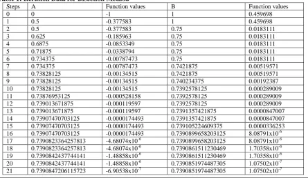
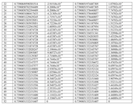
on [0,1], using the software, Mathematica 9.0. The results are presented in Table 1 to 3.Table 1: Iteration Data for Bisection Method
Steps A Function values B Function values
0 0 -1 1 0.459698
1 0.5 -0.377583 1 0.459698
2 0.5 -0.377583 0.75 0.0183111
3 0.625 -0.185963 0.75 0.0183111
4 0.6875 -0.0853349 0.75 0.0183111
5 0.71875 -0.0338794 0.75 0.0183111
6 0.734375 -0.00787473 0.75 0.0183111
7 0.734375 -0.00787473 0.7421875 0.00519571
8 0.73828125 -0.00134515 0.7421875 0.00519571
9 0.73828125 -0.00134515 0.740234375 0.00192387
10 0.73828125 -0.00134515 0.7392578125 0.000289009
11 0.73876953125 -0.000528158 0.7392578125 0.000289009
12 0.739013671875 -0.000119597 0.7392578125 0.000289009
13 0.739013671875 -0.000119597 0.7391357421875 0.0000847007
14 0.73907470703125 -0.0000174493 0.7391357421875 0.0000847007
15 0.73907470703125 -0.0000174493 0.739105224609375 0.0000336253
16 0.73907470703125 -0.0000174493 0.7390899658203125 8.08791x10⁻⁶
17 0.7390823364257813 -4.68074x10⁻⁶ 0.7390899658203125 8.08791x10⁻⁶
18 0.7390823364257813 -4.68074x10⁻⁶ 0.7390861511230469 1.70358x10⁻⁶
19 0.7390842437744141 -1.48858x10⁻⁶ 0.7390861511230469 1.70358x10⁻⁶
20 0.7390842437744141 -1.48858x10⁻⁶ 0.7390851974487305 1.07502x10⁻⁷
22 0.7390849590301514 -2.91518x10⁻⁷ 0.7390851974487305 1.07502x10⁻⁷
23 0.7390850782394409 -9.2008x10⁻⁸ 0.7390851974487305 1.07502x10⁻⁷
24 0.7390850782394409 -9.2008x10⁻⁸ 0.7390851378440857 7.74702x10⁻⁹
25 0.7390851080417633 -4.21305x10⁻⁸ 0.7390851378440857 7.74702x10⁻⁹
26 0.7390851229429245 -1.71917x10⁻⁸ 0.7390851378440857 7.74702x10⁻⁹
27 0.7390851303935051 -4.72236x10⁻⁹ 0.7390851378440857 7.74702x10⁻⁹
28 0.7390851303935051 -4.72236x10⁻⁹ 0.7390851341187954 1.51233x10⁻⁹
29 0.7390851322561502 -1.60501x10⁻⁹ 0.7390851341187954 1.51233x10⁻⁹
30 0.7390851331874728 -4.63387x10⁻¹¹ 0.7390851341187954 1.51233x10⁻⁹
31 0.7390851331874728 -4.63387x10⁻¹¹ 0.7390851336531341 7.32998x10⁻¹⁰
32 0.7390851331874728 -4.63387x10⁻¹¹ 0.7390851334203035 3.43329x10⁻¹⁰
33 0.7390851331874728 -4.63387x10⁻¹¹ 0.7390851333038881 1.48495x10⁻¹⁰
34 0.7390851331874728 -4.63387x10⁻¹¹ 0.7390851332456805 5.10784x10⁻¹¹
35 0.7390851331874728 -4.63387x10⁻¹¹ 0.7390851332165767 2.36988x10⁻¹²
36 0.7390851332020247 -2.19844x10⁻¹¹ 0.7390851332165767 2.36988x10⁻¹²
37 0.7390851332093007 -9.80727x10⁻¹² 0.7390851332165767 2.36988x10⁻¹²
38 0.7390851332129387 -3.71869x10⁻¹² 0.7390851332165767 2.36988x10⁻¹²
39 0.7390851332147577 -6.7446x10⁻¹³ 0.7390851332165767 2.36988x10⁻¹²
40 0.7390851332147577 -6.7446x10⁻¹³ 0.7390851332156672 8.47655x10⁻¹³
41 0.7390851332147577 -6.7446x10⁻¹³ 0.7390851332152124 8.65974x10⁻¹⁴
42 0.7390851332149850 -2.93876x10⁻¹³ 0.7390851332152124 8.65974x10⁻¹⁴
43 0.7390851332150987 -1.03584x10⁻¹³ 0.7390851332152124 8.65974x10⁻¹⁴
44 0.7390851332151556 -8.54872x10⁻¹⁵ 0.7390851332152124 8.65974x10⁻¹⁴
45 0.7390851332151556 -8.54872x10⁻¹⁵ 0.7390851332151840 3.90799x10⁻¹⁴
46 0.7390851332151556 -8.54872x10⁻¹⁵ 0.7390851332151698 1.53211x10⁻¹⁴
47 0.7390851332151556 -8.54872x10⁻¹⁵ 0.7390851332151627 3.44169x10⁻¹⁵
48 0.7390851332151591 -2.55351x10⁻¹⁵ 0.7390851332151627 3.44169x10⁻¹⁵
49 0.7390851332151591 -2.55351x10⁻¹⁵ 0.7390851332151609 4.44089x10⁻¹⁶
50 0.7390851332151600 -1.11022x10⁻¹⁵ 0.7390851332151609 4.44089x10⁻¹⁶
51 0.7390851332151605 -3.33067x10⁻¹⁶ 0.7390851332151609 4.44089x10⁻¹⁶
52 0.7390851332151607 0 0.7390851332151607 0
Table 1 shows the iteration data obtained for Bisection method with the aid of Mathematica 9.0. It was observed that in Table 1 that using the Bisection method, the function, f(x) = x-cosx = 0 at the interval [0,1] converges to 0.7390851332151607 at the 52 second iterations with error level of 0.000000.
Table 2: Iteration Data for Newton- Raphson Method with xo = 0.5.
Steps xk f(xk+1)
1 0.5 -9.62771
2 -9.62771 -2.43009
3 -2.43009 2.39002
4 2.39002 0.535581
5 0.535581 0.750361
6 0.750361 0.739113
7 0.739113 0.739085
8 0.739085 0.739085
Table 2 revealed that with xo=0.5, the function converges to 0.739085 the 8th iteration with error 0.000000.
Table 3: Iteration Data for the Secant Method with [0,2]
xo 0
x1 1
x2 0.685073
x3 0.736299
x4 0.739119
x5 0.739085
x6 0.739085
x7 0.739085
Comparing the results of the three methods under investigation, we observed that the rates of convergence of the methods are in the following order: Secant method > Newton-Raphson method > Bisection method. This is in line with the findings of [4]. Comparing the Newton-Raphson method and the Secant method, we noticed that theoretically, Newton’s method may converge faster than Secant method (order 2 as against α=1.6 for Secant). However, Newton’s method requires the evaluation of both the function f(x) and its derivative at every iteration while Secant method only requires the evaluation of f(x). Hence, Secant method may occasionally be faster in practice as in the case of our study. (see Tables 2 and 3). In Ref. [10-11], it was argued that if we assume that evaluating f(x) takes as much time as evaluating its derivative, and we neglect all other costs, we can do two iterations of Secant (decreasing the logarithm of error by factor α2 =2.6) for the same cost as one iteration of Newton-Raphson method (decreasing the logarithm of error by a factor 2). So, on this premises also, we can claim that Secant method is faster than the Newton’s method in terms of the rate of convergence.
V. CONCLUSION
Based on our results and discussions, we now conclude that the Secant method is formally the most effective of the methods we have considered here in the study. This is sequel to the fact that it has a converging rate close to that of Newton-Raphson method, but requires only a single function evaluation per iteration. We also concluded that though the convergence of Bisection is certain, its rate of convergence is too slow and as such it is quite difficult to extend to use for systems of equations.
REFERENCE
[1] Biswa Nath Datta (2012), Lecture Notes on Numerical Solution of root Finding Problems. www.math.niu.edu/dattab.
[2] Iwetan, C.N, Fuwape,I.A, Olajide, M.S and Adenodi, R.A(2012), Comparative Study of the Bisection and Newton Methods in solving for Zero and Extremes of a Single-Variable Function. J. of NAMP vol.21pp173-176.
[3] Charles A and W.W Cooper (2008), Non-linear Power of Adjacent Extreme Points Methods in Linear Programming, Econometrica Vol. 25(1) pp132-153.
[4] Srivastava,R.B and Srivastava, S (2011), Comparison of Numerical Rate of Convergence of Bisection, Newton and Secant Methods. Journal of Chemical, Biological and Physical Sciences. Vol 2(1) pp 472-479.
[5] Ehiwario, J.C (2013), Lecture Notes on MTH213: Introduction to Numerical Analysis, College of Education Agbor. An Affiliate of Delta State University, Abraka.
[6] http://www.efunda.com/math/num_rootfinding-cfm February,2014 [7] Wikipedia, the free Encyclopedia
[8] Autar, K.K and Egwu, E (2008), http://www.numericalmethods.eng.usf.edu Retrieved on 20th February, 2014.
[9] McDonough, J.M (2001), Lecture in Computationl Numerical Analysis . Dept. of Mechanical Engineering, University of Kentucky.