Auto Regressive Process (1) with Change Point: Bayesian Approch

ISSN (Online): 2320-9364, ISSN (Print): 2320-9356

www.ijres.org Volume 5 Issue 1 ǁ January. 2017 ǁ PP. 27-31

Auto Regressive Process (1) with Change Point: Bayesian

Approch

Dr. Mayuri Pandya, Paras Sheth

Department of Statistics, Maharaja Krishnkumarsinhji Bhavnagar University, Bhavnagar, Gujarat, India.

Abstract :

Here we consider first order autoregressive process with changing autoregressive coefficient at some point of time m. This is called change point inference problem. For Bayes estimation of m and autoregressive coefficient we used MHRW (Metropolis Hasting Random Walk) algorithm and Gibbs sampling. The effects of prior information on the Bayes estimates are also studied.

Keywords:

Auto Regressive Model (1), Bayes Estimator, Change Point, Gibbs Sampling and MHRW Algorithm.

I. INTRODUCTION

Mayuri Pandya (2013) had studied the Bayesian analysis of the autoregressive model Xt = β1 Xt-1 + εt ,

t=1,2,…,m and Xt = β2 Xt-1 + εt , t=m+1,…,n where 0 < β1, β2 < 1, and εt was independent random variable with

an exponential distribution with mean θ1 and is reflected in the sequence after εm is changed in mean θ2. M.

Pandya, K. Bhatt, H. Pandya, C. Thakar (2012) had studied the Bayes estimators of m, β1 and β2 under

Asymmetric loss functions namely Linex loss & General Entropy loss functions of changing auto regression process with normal error. Tsurumi (1987) and Zacks (1983) are useful references on structural changes.

II.

PROPOSED AR (1) MODEL:

Let our AR(1) model be given by,

𝑋𝑖=

𝛽1𝑋𝑖−1 + 𝜖𝑖, 𝑖 = 1,2, … , 𝑚.

𝛽2𝑋𝑖−1+ 𝜖𝑖, 𝑖 = 𝑚 + 1, … , 𝑛.

(1)

where, 𝛽1 and 𝛽2 are unknown autocorrelation coefficients, 𝑥𝑖 is the ith observation of the dependent variable,

the error terms 𝜖𝑖 are independent random variables and follow a N( 0, 𝜎12) for i=1,2,…,m and a N( 0, 𝜎22) for i=

m+1, …..,n and 𝜎12and 𝜎22 both are known. m is the unknown change point and 𝑥0 is the initial quantity.

III.

BAYES ESTIMATION

The Bayes procedure is based on a posterior density, say, g 𝛽₁,𝛽₂,𝑚 | 𝑍 , which is proportional to the product of the likelihood function L 𝛽₁,𝛽₂,𝑚 | 𝑍 , with a joint prior density, say, g 𝛽₁,𝛽₂,𝑚 representing uncertainty on the parameters values.

The likelihood function of β1, β2 and m, given the sample information Zt = (xt-1, xt), t = 1, 2,..., m,

m+1,..., n. is,

𝐿 𝛽1, 𝛽2, 𝑚|𝑍 = 𝐾1 . 𝑒𝑥𝑝 −

1 2𝛽1

2 𝑆𝑚1

𝜎12

+ 𝛽1

𝑆𝑚2

𝜎12

−𝐴1𝑚 2𝜎12

. 𝑒𝑥𝑝 −1 2𝛽2

2 𝑆𝑛1− 𝑆𝑚1

𝜎22

+ 𝛽2

𝑆𝑛2− 𝑆𝑚2

𝜎22

− 𝐴2𝑚 2𝜎22

𝜎1−𝑚 𝜎2 −(𝑛−𝑚 )

(2) Where,

𝑆𝑘1 = xi−12 k

i=1

𝑆𝑘2= xi xi−1 k

i=1

𝐴1𝑚= xi2 m

i=1

𝐴2𝑚 = xi2 n

i=m+1

𝑘1= (2𝜋)− 𝑛 2

3.1Using Informative (Normal) Priors On 𝜷1, 𝜷2

In this section, we derive posterior density of change point m, β1 and β2 of the model explained in

equation (1) under informative priors.

We consider the AR(1) model shown in equation (1) with unknown 𝜎−2_{. We suppose uniform prior of}

change point same as Broemeling (1987), we also suppose that m, β1 and β2 are independent.

𝑔 𝑚 = 1 𝑛 − 1 We have normal prior density on β1 and β2 as,

𝑔 𝛽1 =

1 2𝜋𝑎1 𝑒− 1 2 𝛽1 𝑎1 2

𝑔 𝛽2 =

1 2𝜋𝑎2 𝑒− 1 2 𝛽₂ 𝑎2 2

Hence, joint prior p.d.f. of β1, β2 and m, say g( β1,β2, m) is Joint prior density of 𝛽1, 𝛽2 and 𝑚 Say

𝑔 𝛽1, 𝛽2, 𝑚 is

𝑔 𝛽1, 𝛽2, 𝑚 = 1 2𝜋𝑎₁𝑎₂ 𝑛−1 𝑒

− 1₂ 𝛽 1

𝑎 1 2 𝑒− 1 2 𝛽 2 𝑎 2 2 (4)

Using Likelihood function (2) with the joint prior density (4), the joint posterior density of 𝛽1, 𝛽2, 𝑚 say

𝑔(𝛽1, 𝛽2, 𝑚|𝑍) is,

𝑔 𝛽1, 𝛽2, 𝑚|𝑍 =

𝐾1

ℎ1 𝑧

𝐿 𝛽1, 𝛽2, 𝑚|𝑍 . 𝑔 𝛽1, 𝛽2, 𝑚

= 𝐾2

ℎ1 𝑧

𝑒 − 12 𝛽12𝐴1 + 𝛽1𝐵1 _𝑒 − 1₂ 𝛽22𝐴2+ 𝛽2 𝐵2 _𝑒 −

𝐴_1𝑚 2𝜎₁2 +

𝐴_2𝑚 2𝜎₂2

𝜎1−𝑚 𝜎2 −(𝑛−𝑚 )

(5) Where,

𝐾2= 𝐾1

2𝜋 𝑎1𝑎2 𝑛−1

𝐴1= 𝑆𝑚 1

𝜎12+

1

𝑎12 𝐵1=

𝑆𝑚 2

𝜎12

𝐴2= 𝑆_{𝑛 1}−𝑆_{𝑚 1}

𝜎22 +

1

𝑎22 𝐵2=

𝑆_{𝑛 2}−𝑆_{𝑚 2}

𝜎22 (6)

ℎ1 𝑍 is the marginal density of 𝑧given by,

ℎ1 𝑍 = 𝑛−1𝑚 =1 𝐿 𝛽_{𝛽1 𝛽2} 1, 𝛽2, 𝑚 | 𝑋 . g 𝛽1, 𝛽2, 𝑚 𝑑𝛽1𝑑𝛽2

= 𝑒 −

𝐴 1𝑚 2𝜎 12 +

𝐴 2𝑚

2𝜎 22 _𝜎1−𝑚 _𝜎

2 −(𝑛−𝑚 )

𝑒 −

1 2 𝛽1

2_𝐴 1 + 𝛽1𝐵1 ∞

−∞ 𝑑𝛽1 𝑒

−1

2 𝛽2 2_𝐴

2+ 𝛽2 𝐵2 ∞

−∞ 𝑑𝛽2

𝑛−1

𝑚 =1

= 𝑘3 𝑛−1𝑚 =1𝑇1(𝑚) (7)

Where,

𝑇1 𝑚 = 𝑘𝑚𝐺1𝑚𝐺2𝑚 (8)

𝐺1𝑚 = exp −

1 2 𝛽1

2

𝐴1 + 𝛽1𝐵1 𝑑𝛽1

∞

−∞

=𝑒

𝐵₁2 2𝐴1 _2𝜋

𝐴1

(9)

𝐺2𝑚 = exp −

1 2 𝛽2

2_𝐴

2+ 𝛽2 𝐵2 𝑑𝛽2

∞

−∞

=𝑒

𝐵22

2𝐴_{2 2𝜋}

𝐴2

(10)

𝑘𝑚 = 𝑒 − 𝐴1𝑚

2𝜎12 +

𝐴2𝑚

2𝜎22 𝜎1 −𝑚 _𝜎

2 −(𝑛 −𝑚 )

(11)

Marginal posterior density of change point m, 𝛽1𝑎𝑛𝑑 𝛽2are,

𝑔1(𝑚|𝑥) =

𝑇1(𝑚)

𝑇1(𝑚) 𝑛−1 𝑚 =1

(12)

𝑔1 𝛽1|𝑋 =

𝑘3

ℎ1(𝑋)

𝑘𝑚𝑒

− 1

2 𝛽12𝐴1 + 𝛽1𝐵1

𝑛 −1

𝑚 =1

𝐺1𝑚 (13)

𝑔1 𝛽2|𝑋 =

𝑘3

ℎ1(𝑋)

𝑘𝑚 𝑒 −

1

2 𝛽22𝐴2+ 𝛽2 𝐵2

𝑛 −1

𝑚 =1

𝐺2𝑚 (14)

𝐺1𝑚 ,𝐺2𝑚 and 𝑘𝑚 are define as shows in equation (9), (10) and (11) respectively.

Now, the Bayes estimator of any function of parameter 𝛼, say 𝑔(𝛼) under the squared loss function is, 𝑬𝜶|𝒛 𝒈 𝜶 𝒁 = 𝜶 𝒈 𝜶 𝒁

∞

𝟎 𝒅𝜶 (*)

Gibbs Sampling algorithm:

Given a posterior distribution g(α|Z) for unknown parameters α=( α1,…, αk) defined, at least up to

proportionality, by multiplying the likelihood function with the corresponding prior distribution, we can easily identify the full conditional distribution g(αi|Z, αj,j≠i), upto proportionality, by regarding g(α|Z) as a function of

αi(i=1,…,k) only, corresponding all other αj, j≠i, to be fixed.

To implement the Gibbs sampling procedure, we re-write (13) as full conditional of 𝜷𝟏, by fixing all other

parameters i.e. 𝜷𝟐 and m. Hence full conditional density of 𝜷𝟏 given 𝜷𝟐and m is as follows,

𝑔(𝛽1 | 𝛽2, 𝑚, 𝑍) ∝ 𝑁 𝐵1

𝐴1 ,

1 𝐴1

2

(15)

where A1 and B1 shows in equation (6).

We re-write (14) as full conditional density of β2 by fixing all other parameters β1 and m, we get the full conditional density of β2 given β1, 𝜎-2

and m is as follows, 𝑔(𝛽2 | 𝛽1, 𝑚, 𝑍) ∝ 𝑁

𝐵2

𝐴₂ , 1 𝐴2

2

(16)

where A2 and B2 shows in equation (6).

In order to estimate the parameter 𝛽1, and 𝛽2 we use Gibbs sampling to generate sample from the full

conditional density of 𝛽1 and 𝛽2 given respectively in (15) and (16). We use following algorithm:

Algorithm:

Initialize 𝛽1= 𝛽10, 𝛽2= 𝛽20 and 𝑚 = 𝑚0 then,

Step-1: Generate 𝛽1~𝑁 𝐴1

𝐵₁, 1 𝐵1

2

, using Gibbs Sampling.

Step-2: Generate 𝛽2~𝑁 𝐴₂ 𝐵2,

1 𝐵2

2

, using Gibbs Sampling.

Step-3: Repeat the above steps.

mcmc techniques:

Since the posterior distribution of change point (12) has no closed form, we propose to use MCMC techniques to generate the samples from the posterior distribution. To implement the MCMC Techniques, we re-write (12) as target function of m, by fixing all other parameters i.e. 𝜷𝟏 and . Hence target function of m given 𝜷𝟏 and is as follows,

𝑔 𝑚 𝛽1, 𝛽2 , 𝑍 ∝ 𝑘𝑚 𝑒 − 1

2 𝛽1 2_𝐴

1 + 𝛽1𝐵1 _𝑒 − 1₂ 𝛽22𝐴2 + 𝛽2𝐵2 ₍₁₇₎

where A1, B1,A2B2 𝑎𝑛𝑑 𝑘𝑚shows in equation (6) and (11) respectively.

IV.

NUMERICAL STUDY

Application To Generated Data

Let us consider AR(1) model as

𝑋1=

0.1𝑋𝑖−1 + ∈𝑖 , 𝑖 = 1, 2, … 10

0.3 𝑋𝑖−1+ ∈𝑖 , 𝑖 = 11, 12, . . .20 (18)

Where, the error terms 𝜖𝑖 are independent random variables and follow a 𝑁( 0,1) for i=1,2,…,10. and a 𝑁(0,4)

for i= 11, …..,20 and 𝜎12and 𝜎22known. m is the unknown change point and 𝑥0 = 0.1 is the initial quantity. We

have generated 20 random observations from proposed AR(1) model given in (18). The first ten observations are from normal distribution with 𝜎12= 1 and next 10 are from normal distribution with 𝜎22 = 4. β1 and β2

themselves were random observations from normal distributions with prior means 1 = 0.1, 2 = 0.3 and

variancesa1 = 0.1 and a2 =0.1. These observations are given in table-1.

Table -1: Generated observations from proposed AR(1) model.

i 1 2 3 4 5 6 7 8 9 10

Xi 0.167 -0.204 0.399 -0.259 -0.784 -1.058 0.819 0.404 1.215 1.537 ∈𝑖 0.157 -0.221 0.420 -0.299 -0.758 -0.979 0.925 0.322 1.175 1.416 i 11 12 13 14 15 16 17 18 19 20 Xi -3.833 -16.173 9.441 11.857 20.645 1.458 13.249 -9.335 19.812 30.657 ∈𝑖 -4.294 -15.023 14.293 9.025 17.088 -4.734 12.812 -13.310 22.613 24.713

To generate a random sample from (9.3) using the RWM-H algorithm, the selected proposal is uniform (2, 19) same as prior, which is symmetric around 10 with small steps. Since the target function is bounded.

Distribution is U(3, 14). The results are shown in Table 2 for data given in Table1 when given value of β1=0.1,

β2=0.3, 𝜎12=1 and 𝜎22=16.

Table 2: Bayes Estimates of Change point (m) using RWM-H algorithm under SEL

Bounded Selected proposal

Initial distribution

Bayes Estimate of Change Point

(𝑚)

Integer value of Bayes estimate of Change Point

(𝑚) BD(2,19) U(1,19) U(1,19) 8.4 8 BD(2,19) U(2,19) U(2,19) 8.6 9 BD(3,19) U(1,19) U(1,19) 10.3 10 BD(3,19) U(1,19) U(3,14) 10.2 10

We also compute the Bayes estimators of m using RWM-H algorithm for different prior consideration for data given in Table 1. The results are shown in Table 3.

Table 3: Bayes Estimates of Change point (𝑚) using RWM-H algorithm under SEL for different prior consideration.

Sr. No. 𝑎12 𝑎22

Bayes Estimate of change point (m) (Posterior Mean)

1 0.0100 0.01 10

2 0.0400 0.04 10

3 0.0490 0.04 10

4 0.0550 0.09 10

5 0.0600 0.25 10

6 0.0625 0.49 10

7 0.0900 0.64 10

8 0.4900 0.81 10

9 0.8100 1.00 10

10 1.0000 4.00 10

Now we compute the Bayes estimators of β1 (when given value of β2=0.3, m=10, 𝜎1 2

=1 and 𝜎2 2

=16) and β2 (when given value of β1=0.1, m=10, 𝜎12 =1 and 𝜎22 =16) using Gibbs sampling MCMC algorithm for

different prior consideration for data given in Table 1. The results are shown in Table 4.

Table 4: Bayes Estimates of β1 and β2 using Gibbs Sampling MCMC algorithm under SEL for different prior

consideration.

Sr. No. 𝑎12 𝑎22

Bayes Estimates of S.D. of Bayes Estimates of β1 β2 β1 β2

1 0.0100 0.01 0.025 0.255 0.048 0.008 2 0.0400 0.04 0.090 0.305 0.048 0.008

3 0.0490 0.04 0.107 0.305 0.048 0.008

4 0.0550 0.09 0.118 0.344 0.048 0.008 5 0.0600 0.25 0.126 0.367 0.048 0.008 6 0.0625 0.49 0.130 0.374 0.048 0.008 7 0.0900 0.64 0.172 0.376 0.048 0.008 8 0.4900 0.81 0.415 0.377 0.048 0.008 9 0.8100 1.00 0.475 0.378 0.048 0.008 10 1.0000 4.00 0.496 0.381 0.048 0.008

Figure 1 graph the full conditional of 𝛽1 when a sample of size 10000 is generated from (9.1), Gibbs Sampling

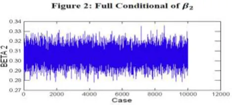
Figure 2 graph the full conditional of 𝛽2 when a sample of size 10000 is generated from (9.2), Gibbs Sampling

with MCMC algorithm has been run. (β1=0.1, m=10, 𝜎12 =1 & 𝜎22 =16)

REFERENCES

[1]. Broemeling, L.D. and Tsurumi, H. (1987), Econometrics and structural change, Marcel Dekker, New York.

[2]. Zacks, S. (1983), Survey of classical and Bayesian approaches to the change point problem: fixed sample and sequential procedures for testing and estimation. Recent advances in statistics. Herman Chernoff Best Shrift, Academic Press New-York, 1983, 245-269.

[3]. M. Pandya, K. Bhatt & H. Pandya, C. Thakar (2012), Bayesian estimation of change point in autoregressive process, IJRRAS 13 (1).

[4]. M. Pandya, H. Pandya & S. Pandya (2012), Bayesian inference on mixture of geometric with degenerate distribution: zero inflated geometric distribution, IJRRAS 13 (1).