A novel feature selection algorithm based on
hypothesis-margin
Ming Yang* Fei Wang and Ping Yang
Department of Computer Science, Nanjing Normal University, Nanjing, P.R.China Email: {m.yang, yangping}@njnu.edu.cn, [email protected]
Abstract—Iterative search margin based algorithm(Simba) has been proven effective for feature selection. However, it still has the following disadvantages: (1) the previously proposed model still lacks enough robust to noises; and (2) the given model does not use any global information, in this way some useful discrimination information may be lost and the convergence speed is also influenced in some cases. In this paper, by incorporating global information, a novel margin based feature selection framework is introduced. According to the newly designed model, an improved margin based feature selection algorithm(Isimba) is proposed. By effectively adjusting the contribution of the global information, Isimba can efficiently reduce the computational cost and at the same time obtain more effective feature subsets as compared to Simba. The experiments on 6 artificial and 8 real-life benchmark datasets show that Isimba is effective and efficient.
Index Terms—Feature selection, Dimensionality reduction, Hypothesis-margin, Margin
I. INTRODUCTION
Dimensionality reduction(DR) is one commonly applied approach[1]. There are a number of DR technique, and according to the adopted reduction strategy, they are usually divided into feature extraction[2-4] and feature selection[5] approaches. The key difference between feature extraction and feature selection is that the former one is based on generation of a completely new feature space through a functional transforming, while the latter one is to select a relevant subset of original features. The classical feature extraction methods are generally classified into linear and nonlinear methods. Linear approaches, such as Principal Component Analysis (PCA)[2], and Linear Discriminant Analysis (LDA)[1] and Locality Preserving Projections(LPP)[3], aim to project the high-dimensional data to a lower-dimensional space by linear transformations according to some criteria. On the other hand, nonlinear methods, such as Locally Linear Embedding(LLE)[4] aims to project the original data by nonlinear transformations while preserving certain local information according to some criteria. As authors of Ref.[5] pointed out, feature extraction is
generally effective. However, the effectiveness of the feature extraction algorithms may be obviously degraded when processing large-scale data sets. In addition, new variables usually concern with all original features, so forming new variables may contain lots of information originated from those redundant features in the original space, such as PCA[2].
Unlike feature extraction, feature selection can be viewed as one of the most fundamental problems in machine learning field. It is defined as a process of selecting relevant features out of the larger set of candidate features. The relevant features are defined as features that describe the target task. As Liu pointed out in [6], the motivation of feature selection(also called attribute reduction or feature reduction) in data mining and machine learning is to: reduce the dimensionality of feature space, speed up and reduce the cost of a learning algorithm, improve the predictive accuracy of a classification algorithm, and to improve the visualization and the comprehensibility of the induced concepts. Especially, the authors of [6] have emphasized that not every feature selection method can serve all purposes.
Generally, supervised feature reduction methods can be categorized into two classes: the filter model [7-9][12][13]and the wrapper model[10][11][14]. In the wrapper model the feature selection methods try to directly optimize the performance of a specific predictor. Along this, the predictor generalization performance (e.g. by cross validation) needs to be estimated for the selected feature subset in each step. So, high computational cost is its main disadvantage.
Currently, there are many filter methods available, including Relief [7],FCBF [8], C-tree based feature selection algorithm[9] and Simba[12], etc. Among them, Simba is the recently proposed margin based feature selection approach, which uses the so-called large margin principle[15-16] as its theoretical foundation to guarantee good performance for any feature selection scheme which selects small set of feature while keeping the margin large. Meanwhile, by the smoothness of the hypothesis-margin based evaluation function, Simba uses a stochastic gradient ascent over the evaluation function to accelerate the feature selection process. Roughly speaking, the main idea of Simba is to obtain an effective subset of features such that the relatively significant features have relatively large weights by using hypothesis-margin criterion. In *Corresponding author. Tel.: +86-25-51912532; fax:+86-25-83598391.
essence, similar to Ref.[14], Simba is also a weighted method, that is, those features with relatively larger weights form the subset of features, but the key difference is that Simba is filter method and most of the other weighted methods are related to a concrete classifier. Moreover, theoretical analysis and experiments show that Simba can effectively reduce the computational complexity and is more effective than the classical filter approach, such as Relief[7].
However, one disadvantage of Simba is its non-robustness to noises, that is, the weights of some features by the effect of noises may become relatively larger or may not converge to a relatively small value or zero by using 1NN criterion[17][18], since noises may increase the contribution of some features to the hypothesis-margin of samples. On the other hand, Simba only uses local information for choosing a small set of features to make the hypothesis-margin of samples large, in this way it may lose some useful discrimination information or global structure hidden in the global information. Thus, the performance of classifiers induced by post-analysis algorithms in the new feature space will be degraded.
In this paper, we introduce a novel margin based feature selection model called Isimba_FS which incorporates the global information into the recently proposed margin based feature selection model[12] to eliminate the disadvantages of Simba algorithm while maintaining its merits. In Isimba_FS, the main motivation incorporating global information attempts to make the distance between a sample and the center point with same class as small as possible and the distance between a sample and the center point with different classes as large as possible, and meanwhile a balance factor λ is introduced for dynamically adjusting the contribution of global information. Along the newly designed model Isimba_FS, we introduce an improved margin based feature selection algorithm (Isimba). By adjusting the contribution of the global information, Isimba can efficiently reduce the computational cost and meanwhile get a more effective feature subset as compared to Simba. In summary, Isimba possesses several attractive characteristics as follows: (1) the computational complexity can be efficiently reduced, since the centers of each class and remaining classes can be computed in advance, and their contributions to the weight vector can be reflected at each iteration; (2) the classification performance of classifiers induced by the selected small set of features can be effectively improved in some cases because the embedded global information can guarantee both discrimination information-preserving and noises-resisting; and (3) the contribution of global information can be dynamically adjusted effectively by the tradeoff parameter λ.
The rest of this paper is organized as follows. In Section 2, some basic concepts on margin(hypothesis-margin and sample-margin(hypothesis-margin) and Simba are briefly introduced. In Section 3, by incorporating global information into the existing feature selection model based on hypothesis-margin, a novel feature selection model and corresponding feature selection algorithm are
presented. Some experimental comparisons are introduced in Section 4. Finally, Section 5 gives our conclusions and several issues for future works.
II. PRELIMINARIES
A. SAMPLE-MARGIN AND AND HYPOTHESIS-MARGIN
As authors of Ref.[12] pointed out, margins play a crucial role in modern machine learning research. They measure the classifier confidence when making its decision. Margins are used for theoretic generalization bounds and as guidelines for algorithm design.
As described in Ref.[15], there are two natural way of defining the margin of a sample with respect to a classification rule. The more common type, sample-margin, measures the distance between the sample and the decision boundary induced by the classifier, e.g., Support Vector Machine (SVM)[16] finds the separating hype-plane with the largest sample-margin. Obviously, those feature selection methods based on sample-margin need high computational cost for large-scale or/and high-dimensional data sets.
So, as an alternative definition, the hypothesis-margin was introduced in [12][15]. The margin of a hypothesis with respect to a sample is the distance between the hypothesis and the closest hypothesis that assigns alternative label to the given sample. The hypothesis-margin of a sample x for 1NN with respect to a set to samples P is defined as follows.
1
( ) (|| ( ) || || ( ) ||)
2
P nearmiss nearhit
θ x = x− x − x− x (1)
where nearhit(x) and nearmiss(x) denote the nearest sample to x in P with the same and different label, respectively. By (1), we hope to choose a subset of original features such that the hypothesis-margin becomes as large as possible. Based on hypothesis-margin, the effective feature subset can be efficiently obtained by corresponding feature selection algorithms, since in the case of Nearest Neighbor large hypothesis-margin can ensures largesample-margin, and hypothesis-margin is easy to compute as comparing to sample-margin.
B. EVALUATION FUNCTION
In order to obtain the more effective subset of original features, an evaluation function which assigns a score to sets of features according to the hypothesis-margin they induce was introduced in Ref.[12], the hypothesis-margin as a function of the chosen set of features is formulated as following Definition 1.
Definition 1[12]. Let P be a set of samples and x be a sample. Let w be a weight vector over the feature set, then the hypothesis-margin of x is
1 (|| ( ) || || ( ) || )
2
P nearmiss nearhit
θw= − − −
w w
x x x x (2)
where || || 2 2
Further, by (2), the authors of Ref.[12] provide a strategy for computing the hypothesis-margin of all the given samples by following Definition 2.
Definition 2[12]. Given a training set S and a weight vector w, the evaluation function is
( ) ( { })S ( ) S
e θ −
∈ ∑
= w
x x
w x (3)
By (3), the feature set can be found by maximizing the hypothesis-margin directly, that is, the weight vector w that maximizes e(w) as defined in (3) is first found. Then, let max 2
i
w =1, the corresponding normalization weight
vector w can be obtained, hence a subset of features can be naturally gotten by using a threshold.
C. ITERATIVE SEARCH MARGIN BASED ALGORITHM
In order to quickly and effectively obtain a subset of original features, the so-called gradient ascent strategy was employed in [12] for maximizing e(w) as defined in (3), since e(w) is smooth almost everywhere. The gradient of e(w) when evaluated on the set of samples S is
2 2 ( ) ( ) ( ( )) ( ( ) ) ( ( ) ) 1 ( )
2 || ( ) || || ( ) ||
i
S
i i
i i i i
i S w w e e w w nearmiss nearhit w nearmiss nearhit θ ∈ ∈ ∑ ∑ ∂ ∂ ∇ = = ∂ ∂ − − = − − − x x w x w
x x x x
x x x x
(4)
As described above, the description of the iterative search margin based algorithm for feature selection is as follows.
Algorithm 1. Simba[12] 1. initialize w=(1,1,…,1); 2. for t=1,2,…,T;
(a) pick randomly a sample x from S;
(b) calculate nearmiss(x) and nearhit(x) with respect to (S−{x}) and the weight vector w;
(c) for i=1,2,…,N calculate
2 2
( ( ) ) ( ( ) )
1 ( )
2 || ( ) || || ( ) ||
i i i i
i i nearmiss nearhit w nearmiss nearhit − − ∆ = −
− w − w
x x x x
x x x x
(d) w= + ∆w 3. 2/ || 2||
∞
←
w w w when ( ) : ( )w2 i = wi 2.
Since ||w|| increases, the relative effect of the correction term ∆decreases and the algorithm typically convergence. The computational complexity of Simba is O(TNm), where T is the number of iterations, N is the number of features and m is the size of the samples S. Obviously, Simba is in high efficiency. Further, the numerical experiments show that Simba outperforms Relief.
However, Simba only uses the a few local information to calculate the hypothesis-margin of the given samples according to the margin measure of a hypothesis of a sample, in this way some irrelevant features may have relatively larger weights due to the influence of noises, hence Simba is still non-robust. At the same time, Simba cannot use the useful discrimination information hidden in the global information, this may lead to loss of some useful features.
III. ISIMBA_FS AND ISIMBA
In order to overcome the disadvantages of Simba and still retain its characteristics, we propose a novel margin based feature selection model called Isimba_FS incorporating global information. Further, based on Isimba_FS, we introduce an improved margin based feature selection algorithm(Isimba).
A. HYPOTHESIS-MARGIN INCORPORATING GLOBAL INFORMATION
To remedy the shortcomings of Simba algorithm, we introduce a novel margin based feature selection model( Isimba_FS ) incorporating global information as follows. 1 ˆ ( ) (|| ( ) || || ( ) ||) 2 (|| ( ) || || ( ) ||) 2
P nearmiss nearhit
centermiss centerhit
θ λ
= − − −
+ − − −
x x x x x
x x x x
(5)
where nearhit(x) and nearmiss(x) denote the nearest sample to x in P with the same and different label, respectively; centerhit(x) and centermiss(x) denote the centers to x in P with the same and different label, respectively; λ(Lambda) is an adjustable parameter, it is used to control the contribution of global information to the hypothesis-margin described in Section 2. To balance the contributions of local and global information to the hypothesis-margin, in this paper we employ a non-optimized but effective strategy, let λ be selected in {0,0.001,0.01,0.1,0.3,0.5,1,5}.
The novel hypothesis-margin incorporating global information naturally has the following merits:
(1) when λ=0, Eq.(5) degrades to Eq.(1), that is, the new hypothesis-margin model is an extension of the original hypothesis-margin.
(2) when λ >0, all margin based feature selection algorithms induced by Eq.(5) can efficiently reduce the number of iterations to some extent, since in a given samples the centers to any samples with the same and different label can be computed in advance. Moreover, when λ gradually increases, the convergence speed of those feature selection algorithms based on Eq.(5) can be naturally accelerated.
(3) the adjustable parameter λ can effectively adjust the tradeoff between the contributions of local and global information to the new hypothesis-margin. By tuning λ to a relatively larger value, those features preserving the discrimination information or global structure hidden in data and holding larger hypothesis-margin can effectively obtained.
(4) the robustness of the feature selection algorithms induced by Eq.(5) can be effectively enhanced because the embedded global information can constrain the influence of noises to some extent.
B. A NOVEL EVALUATION FUNCTION BASED ON THE NEW HYPOTHESIS-MARGIN
Definition 3. Let P be a set of samples and x be a sample, and w be a weight vector over the feature set, then the new hypothesis-margin of x is
1
ˆ ((|| ( ) || || ( ) || )
2
(|| ( ) || || ( ) || ))
P nearmiss nearhit
centermiss centerhit θ λ = − − − + − − − w w w w w
x x x x
x x x x
(6)
Further, based on this evaluation function, we introduce a strategy for computing the new hypothesis-margin of all the given samples as follows.
Definition 4. Given a training set S and a weight vector w, the new evaluation function is
( { }) ˆ
ˆ( ) S ( )
S
e = ∈∑ θw−x x
w x
(7)
According to Eq.(7), it is also nature to consider the evaluation function only for weight vector w such that
2
maxwi =1. However, similar to (3), we can also ignore the constraint || 2|| 1
∞=
w when computing the weight vector w, since eˆ(βw)=βeˆ( )w . After finding w, let
2
maxwi =1, we normalize the weight vector w and easily
obtain a subset of features by using a threshold.
C. IMPROVED ITERATIVE SEARCH MARGIN BASED ALGORITHM
As analyzed in Section 3.2, we can use the weights directly by using the induced distance measure instead for maximizing eˆ( )w as defined in (7). Also, we can directly use gradient ascent in order to maximize it, since eˆ( )w is smooth almost everywhere. Similar to (4), the gradient of
ˆ( )
ew when evaluated on the set of samples S is as follows.
ˆ ( ( ))∇e w i
ˆ( ) i e w ∂ = ∂
w ˆ( )
x S i x w θ ∈ ∑ ∂ = ∂ 2 2 2 2 ( ( ) ) ( ( ) )
1 ( ( )
2 || ( ) || || ( ) ||
( ( ) ) ( ( ) )
( ))
|| ( ) || || ( ) ||
i i i i
S
i i i i
i S
x nearmiss x x nearhit x x nearmiss x nearhit
x centermiss x x centerhit x w centermiss centerhit λ ∈ ∈ ∑ ∑ − − = − − − − − + − − − x w w x w w x x
x x x x
(8)
By Eq.(8), an improved iterative search margin based algorithm(Isimba) for feature selection is as follows. Algorithm 2. Isimba
1.letλbe a proper non-negative number; 2. initialize w=(1,1,…,1);
3. for each x∈S do
calculate centermiss(x) and centerhit(x), where centermiss(x) and centerhit(x) are the centers to x in P with the same and different label, respectively; 4. for t=1,2,…,T;
(a) pick randomly a sample x from S;
(b) calculate nearmiss(x) and nearhit(x) with respect to (S−{x}) and the weight vector w;
(c) for i=1,2,…,N calculate
2 2
2 2
( ( ) ) ( ( ) )
1
ˆ (( )
2 || ( ) || || ( ) ||
( ( ) ) ( ( ) )
( ))
|| ( ) || || ( ) ||
i i i i
i
w
i i i i
i
w w
x nearmiss x x nearhit x nearmiss nearhit
x centermiss x x centerhit x w centermiss centerhit λ − − ∆ = − − − − − + − − − w
x x x x
x x x x
(d) w= + ∆w ˆ 5. 2/ || 2||
∞ ←
w w w when ( ) : ( )w2 i = wi 2.
In Isimbaalgorithm, we also use a stochastic gradient ascent over eˆ( )w while ignoring the constraint
2
||w ||∞=1, the normalization on the constraint is done only at the step 5, since eˆ(βw)=βeˆ( )w . Moreover, in each iteration we only evaluate one term in the sum in (8) and add it to the weight vector w. In addition, the term ∆ˆ
in step 4(d) is invariant to scalar scaling of w, since ˆ( ) ˆ(β )
∆ w = ∆ w . So, when ||w|| increases gradually, the relative effect of the correction term ∆ˆ decreases and
Isimba typically convergence.
Also, the second term of Eq.(8) can be directly induced by the obtained centermiss(x) and centerhit(x) because both centermiss(x) and centerhit(x) are computed in advance for any given sample x, hence it is easy to see that the contribution of global information to weight vector w almost need not spend any computational cost. Also, in intuitive, when λgradually increases, the effect of global information to the weight vector w also increases naturally, this directly leads to reduction of the number of iterations. So, Isimba algorithm can efficiently reduce the computational cost.
Further, in most cases Isimba algorithm can obtain the more effective subset of features as compared to Simba, since by dynamically adjusting the controlled parameter λ, Isimba makes the global structure or discrimination information hidden in data to be preserved in the new feature space. Especially, when λ=0, Isimba degrades to Simba, hence they can obtain a consistent subset of features in this case, but this is not the optimized result of Isimba. Moreover, by incorporating relevant global information, the robustness of Isimba can be effectively enhanced to some extent. In addition, to select a relatively small feature set, we can still use the same threshold strategy as Ref.[13], namely all features with a relevance score less than the specified threshold are removed, e.g., if the relevant threshold δ (delta) is set to 0.01, all features with the weight less than δ are removed.
In general, by incorporating the global information, Isimba should outperform Simba intuitively. To test the performance of Isimba the related experiments on 6 artificial and 8 real-life datasets will be presented in Section 4.
IV. EXPERIMENTAL RESULTS
and the classification accuracies of the classifiers kNN and SVM based on the new feature subspace.
A. ARTIFICIAL DATASETS
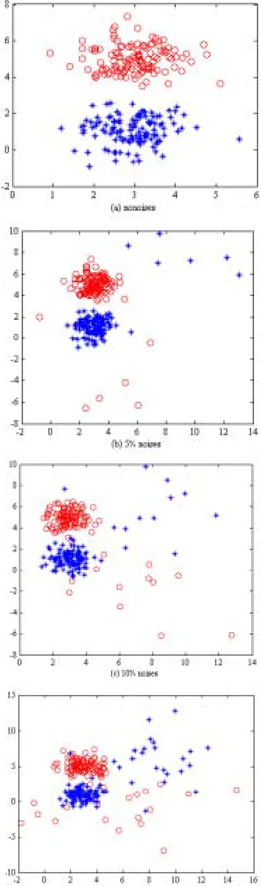
In this subsection, the robustness of Simba and Isimba is testified, here we call a feature selection algorithm is robust enough if the feature subset obtained from the dataset with noises is almost consistent with that generated from the originally pure dataset. For this purpose, we generate one artificial dataset with no noises, dataset1, which is a two-dimensional artificial dataset composed of two classes and 240 samples as shown in Fig. 1(a). The 120 samples in class 1 of the dataset1 are randomly generated from a Gaussian distribution with mean [3,5] and variance diag[0.5,0.5], and the 120 samples in class 2 of the dataset1 are randomly generated from a Gaussian distribution with mean [3,1] and variance diag[0.5,0.5]. Further, in order to examine the robustness of Simba and Isimba, we generate 5 artificial datasets dataset2, dataset3, dataset4, and dataset5 and dataset6 with 5%,10%,20%,25% and 30% noises as seen in Fig.1(b-f) respectively, in which the noise samples in class 1 are randomly generated from a Gaussian distribution with mean [6,-1] and variance diag[10,10], and the noise samples in class 2 are randomly generated from a Gaussian distribution with mean [8,6] and variance diag[10,10].
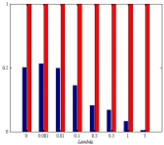
As can be seen in Fig.2, for the given dataset1 with no noises, Simba can effectively filter out the first feature due to its weight less than the given threshold δ (hereδ is set to 0.01). However, from the Fig.2, we can also observe that Simba is non-robust when the noise samples in original dataset is over 5%. Meanwhile, as seen from Figs.3 and 4, when the controlled parameter λincreases gradually, the robustness of Isimba becomes more stronger. That is, the robustness of Isimba can be enhanced by properly adjusting the balance parameter λ. Further, to analyze the connection between the computational cost and global information, we say the algorithm can not effectively eliminate the influence of noises when it repeatedly iterates the given maximum number of iterations but those irrelevant features also holds relatively large weights. In Fig. 5, the maximum number of iterations is set to 3600. From Fig. 5, we observe that the computational cost is efficiently reduced with large λ. At the same time, it also can be seen that we need to incorporate more global information to copy with the influence of noises.
Figure 1. Artificial datasets(dataset1-6)
Figure 2. The weights Simba assigns to the 2 features
Figure 3. The weights ISimba assigns to the 2 features under 10%noises
Figure 4. The weights ISimba assigns to the 2 features under 20%noises
Figure 5. The number of iterations of Isimba
Figure 6. The classification accuracy of KNN(k=5) on Ionosphere
TABLE 1.EXPERIMENTAL RESULTS(δ =0.01) Parameter
dataset FS algorithm
s
λ Nf
3NN 5NN 7NN KSVM
- - 13 94.44 94.44 94.44 97.78
Wine Isimba 0 11 96.67 96.67 96.67
98.89
- - 6 69.36 67.05 64.74 71.68
BLD
Isimba 0,0.1 5 66.47 67.05 68.21 73.41
- - 5 94.44 92.59 92.59 94.44
Tyroid
Isimba 0-0.1 4 92.59 92.59 93.52 96.29
- - 9 92.81 93.22 93.08 92.54
Simba 0 6 92.40 92.13 92.40 92.54 CMC
Isimba 0.1 6 93.22 92.94 93.08 92.54
- - 60 75.24 72.38 66.67 85.71 Simba 0 29 80.00 81.9 73.33 89.52
Sonar
Isimba 0.1 30 82.86 80.95 74.45 87.62
- - 8 71.61 72.92 73.44 78.65
Simba 0 7 69.27 70.83 73.44 78.13 Diabete
Isimba 0.3 5 72.92 73.96 76.30 78.39
- - 34 77.84 73.86 72.16 94.89 Simba 0 9 88.64 85.80 85.80 93.75
Ion
Isimba 0.01 10 84.66 82.39 83.52 94.32
- - 21 79.81 80.13 80.97 86.49 Simba 0 13 80.25 82.05 83.45 85.33
Wave
Isimba 0.01 14 81.25 82.09 83.37 85.53
Notes: “-“ means that no feature selection is done; the cells labeled using blue represent the accuracy of the SVM-based and kNN-based classifiers on original features; the bold face cells denote that kNN-based and/or SVM-based classifiers induced by the chosen feature subsets have
more better or comparable performance.
B. REAL-LIFE DATASETS
In this paper, those employed datasets are the publicly available datasets from UCI database (downloaded at http://www.ics.uci.edu). A brief description for the UCI datasets is given at first: (1) Wine recognition data (Wine) :178 objects, 3-class, 13-features;For short,(178, 3C,13F) (2) BUPA Liver Disorders(BLD): (345,2C,6F); (3)Thyroid: (215,3C,5F); (4) Contraceptive Method Coice (CMC): (1473,2C, 9F); (5) Sonar: (208,2C,60F); (6) Pima Indians Diabetes (Diabete): (768,2C,8F); (7) Ionosphere (Ion):(351,2C, 34F); (8) Waveform domain data (Wave): (5000,3C, 21F).
In our experiments, every dataset is randomly partitioned into two halves: one half is used for training and the other for testing. It is worth noting that all features are normalized to the range between 0 and 1. the balance parameter λ is selected in {0,0.001,0.01, 0.1,0.3,0.5,1,5} for simplicity. To select a relatively small feature set, in this paper the relevant threshold δ is set {0.001, 0.01, 0.05}, all features with their weight less than δ are removed. In addition, let λs denotes the set of
the values of λ that can get the same feature subset when δ is fixed, Nf the number of the selected features. Also,
both Simba and Isimba are independent of post-analysis algorithms (predictors), here we choose well known k -Nearest-Neighbor (kNN)[16][17] and SVM(Support Vector Mahine) with kernels[15] as evaluating criteria for testing the classification accuracy of the chosen feature subset. In the KSVM algorithm, we employ C-SVM model and use RBF kernel as the kernel function.
The experimental results are shown in Table 1 when δ is set to 0.01. From Table 1, we can find that the effective feature subsets could be obtained, and corresponding classifiers have better or comparable performance than those based on original features on all datasets. Further, for those datasets diabete, ionosphere and wave, by
adjusting the balance parameter λ Isimba algorithm can get more effective feature subsets as compared to Simba. So, incorporating appropriately global information is of great benefit to enhancing the performance of the newly developed model.
At the same time, from Table 1, we also find that those effective feature subsets are obtained when λis relatively small, namely it varies within a range around 0.1. This is consistent with our intuitive observation, because for any sample x, it is near to the center point with same label but far to the center point with different label. In other words, as comparing to the contribution of the local information, the global information may have a relatively great effect to the weight vector in most cases. So, a relatively small λcan effectively adjust the trade-off between the local information and global information for getting more effective feature subset.
Further, from the experimental result, we also observe that those very importance features are always kept in the results no matter λis 0 or not 0. This further indicates that Simba is indeed a very important feature selection algorithm. Based on Isimba, by tuning the parameter λ, the weights of some effective features which are filtered out by Simba should be increased. Hence, Isimba is naturally an extension and improvement ofSimba.
It is worth noting that the parameters in Table 1 is not optimized results, since δ is set to a fixed value 0.01, λ is selected in {0,0.001,0.01,0.1,0.3,0.5,1,5}. However, we still need to point out that even so, on all 8 datasets, the classifiers induced by Isimba still achieve better or comparable classification performance as compared to the classifiers established by all features.
C. INFLUENCE OF THE PARAMETERS δ AND λ ON CLASSIFICATION PERFORMANCE
In the above experiment, for a fixed threshold parameter δ , although Isimba can get a more effective feature subset in most cases, this is not optimized results. In order to get a relatively appropriate value of δ , we need to record the performance of the classifiers when δ and λ change. For simplicity of illustration, we just present the value of λ’s impact on the performance of Isimba on the dataset Ionosphere under the different δ , here let δ be set three different values in {0.001,0.01, 0.05}.
It is known that the more features are removed as δ increases, while the more features are chosen when δ decreases. From Figs.6 and 7, we also observe that determining a proper value of δ is also a challenging issue, since the classification accuracy varies unorderly when δ changes orderly under λ is fixed, e.g., as can be seen from Fig.6, the classification accuracy increases from 78.98% to 91.48% as δ varying from 0.001 to 0.05 under λ=0.001, but the classification accuracy decreases from 92.05% to 87.5% as δ varying from 0.001 to 0.05 under λ=0.5. So, we can find that selecting a feature only according to its weight is only relatively effective but not optimized method, because those feature subset with relatively larger weights may contain some irrelevant features. Using the weights of features as baseline, seeking the new strategy to select those more effective features is our ongoing work.
V. CONCLUSIONS AND FUTURE WORK
In this paper, we introduce a novel margin based feature selection model, which effectively incorporates global information into the original hypothesis-margin based feature selection model. In the new model, the contribution of global information can be dynamically adjusted, hence which is an extension of the original model. Further, based on the new hypothesis-margin, a novel feature selection algorithm(Isimba) is introduced. By properly incorporating global information, the newly developed algorithm not only can enhance effectively its robustness to noises, but also can preserve the global structure information hidden in the given data and meanwhile reduce efficiently the computational cost. Consequently, the classification performance of the classifiers followed by establishing the newly proposed algorithm is improved on almost all datasets used here.
On the other hand, experimental results on 8 real-life datasets are summarized as follows: (1) the classifiers induced by the obtained feature subset using Isimba consistently outperform the corresponding classifiers obtained by the all features in classification performance on all the datasets; (2) the balance and threshold parameters λand δ influence the quality of the obtained feature subset, adjusting suitably their values can guarantee to obtain a more effective feature subset; and (3) a relatively large tradeoff parameter λ can efficiently reduce the time complexities of Isimba.
Our further and ongoing works include the adaptive determination of both parameters λand δ , and how to more reasonably use global information.
ACKNOWLEDGMENT
This work was supported in part by National Natural Science Foundation of P.R.China and Jiangsu Province under Grant Nos.60873176 and BK2008430, respectively.
REFERENCES
[1] K.Fukunaga. Introduction of Statistical Pattern Recognition. Second ed. Academic Press, 1991
[2] I.T.Jolliffe. Principal Component Analysis. Second ed. Wiley,2002.
[3] X.He, S.Yan, Y.Hu, et al. Face Recognition Using Laplacianfaces. IEEE TPAMI, 2005,27(3): 328-340
[4] S.Roweis and L.Saul. Nonlinear Dimensionality Reduction by Locally Linear Embedding. Science, 2000,29(22):2323-2326.
[5] J.Yan, B.Y.Zhang, N.Liu, et al. Effective and Efficient Dimensionality Reduction for Large-Scale and Streaming Data Preprocessing. IEEE TKDE, 2006,18(3):320-333 [6] H.Liu and H.Motoda. Feature selection for knowledge
discovery and data mining. Kluwer, Boston,1998.
[7] K.Kira and L.Rendell. A practical approach to feature selection. Proc. 9th Inte. Workshop on Machine Learning, 1992.249-256
[8] L.Yu and H.Liu. Feature selection for high-dimensional data: a fast correlation-based filter solution. In proceedings of ICML 2003.
[9] Ming Yang, Ping Yang. A Novel Condensing Tree Structure for Rough Set feature selection. Neurocomputing, 2008,71(4-6):1092-1100
[10] G.H.John, R.Kohavi and K.Pfleger. Irrelevant feature and the subset selection problem. Proc. of the 11th ICML, Morgan Kaufmann Publishers,San Francisco,CA, 1994.121-129 [11] R.Kohavi & G.John. Wrappers for feature subset selection.
Artificial Intelligence,1997,97(1-2):273-324
[12] Ran Gilad-Bachrach, Amir Navot and Naftali Tishby. Margin Based Feature Selection-Theory and Algorithms. In Proc. of the 21st ICML, Banff, Canada, 2004.43-50
[13] I.Kononenko. Estimating attributes: Analysis and extensions of relief. In Proceedings of the Seventh ECML, Springer-Verlag,1994.171-182.
[14] Isabelle Guyon and André Elisseeff. An Introduction to Variable and Feature Selection. JMLR, 2003(3):1157-1182. [15] K.Crammer, R.Gilad-Bachrach, A.Navot, N.Tishby.
Margin analysis of the lvq algorithm. Proc. of 17th CNIPS, 2002.
[16] V.Vapnik. The nature of statistical learning theory. New York :Springer-Verlag,1995
[17] C.Domeniconi, J.Peng, D.Gunopulos. Locally daptive metric nearest-neighbor classification. IEEE TPAMI,2002, 24(9): 1281-1285.
[18] T. Hastie and R.Tibshirani. Discriminant Adaptive Nearest Neighbor Classification. IEEE TPAMI, 1996, 18(6):607-616