A Parallel Algorithm for Gene Expressing Data
Biclustering
LIU Wei
Institute of Information Science and Technology, Nanjing University of Aeronautics and Astronautics, Nanjing, China Email: [email protected]
CHEN Ling
Department of Computer Science, Yangzhou University, Yangzhou, China
National Key Laboratory of Novel Software Technology, Nanjing University, Nanjing, China Email: [email protected]
Abstract—Biclustering of the gene expressing data is an important task in bioinformatics. By clustering the gene expressing data obtained under different experimental conditions, function and regulatory elements of the gene sequence can be analyzed and recognized. A parallel biclustering algorithm for gene expressing data is presented. Based on the anti-monotones property of the quality of the data sets with their sizes, the algorithm starts from the data sets containing of all the 2*2 submatrices of the gene expressing data matrix, and gets the final biclusters by gradually adding columns and rows on the data sets. Experimental results show that our algorithm has superiority over other similar algorithms in terms of processing speedup and quality of clustering and efficiency.
Index Terms—bioinformatics, biclustering, gene expression data
I. INTRODUCTION
In DNA microarray experiments, a key step in the analysis of gene expression data is to discover groups of genes that share similar transcriptional behavior. Microarray techniques may provide massive amounts of information, which is leading to the development of sophisticated algorithms capable of extracting novel and useful knowledge from a biomedical point of view. Microarray data are widely used in genomic research due to the enormous potential in gene expression profiling, facilitating the prognosis and the discovering of subtypes of diseases. Clustering gene expression data into homogeneous groups is instrumental in functional annotation, tissue classification, motif identification. Gene expression data generated by DNA chips and other microarray techniques are often presented as matrices of expression levels of genes under different conditions including environments, individuals, and tissues. One of the usual goals in expression data analysis is to group genes according to their expression under multiple conditions, or to group conditions based on the expression of a number of genes. This may lead to discovery of regulatory patterns or condition similarities. Clustering has been applied to gene expression data,
which usually refers to conditions or patients, although genes can also be grouped in order to search for functional similarities. The current practice is often the application of some agglomerative or divisive clustering algorithm that partitions the genes or conditions into mutually exclusive groups or hierarchies. The basis for clustering is often the similarity between genes or conditions as a function of the rows or columns in the expression matrix. The similarity between rows is often a function of the row vectors involved and that between columns a function of the column vectors.
However, relevant genes are not necessarily related to every condition or, in other words, there are genes that can be relevant for a subset of conditions. On the contrary, it is also possible to discriminate groups of conditions by using different groups of genes. From this point of view, clustering cannot only be addressed on the conditions or genes, but also in the two dimensions simultaneously. We not only do clustering on gene sequences, but also consider the variety in experimental conditions. Therefore, biclustering of gene expression data is to identify groups of genes that show a “similar” expression level or trend under a specific subset of experimental conditions. In biclustering of gene expression data, we can make clustering analysis through both rows and columns of gene expression matrix and get clustering made up of both subsets of genes and subsets of conditions.
Existing methods for biclustering the gene expressing data can be classified in five categories.
1. Iterative row and column method, such as the Coupled Two-Way Clustering (CTWC) presented by G. Getz[1] et al. Based on pairs of row/column clusters,
CTWC can continuously identify new “stable” row/column through hierarchical clustering. In the Interrelated Two-Way Clustering (ITWC) method proposed by Chun Tang[2] et al., rows are first clustered
the best 1/3 rows in the heterogeneous pairs are kept in each iteration. The iteration would be terminated until certain conditions are satisfied.
2. Divide and conquer method, such as Block Clustering proposed by Hartigan[3] et al. This approach
would first sort the data by row or column mean and then find the best row or column split to reduce “within block” variance. Repeating alternate row or column splits until desired K blocks are obtained. This approach is very fast, but likely to miss biclusters due to early splits.
3. Greedy iterative search method, such as δ-bicluster[4]
approach presented by Cheng & Church et al. , FLOC [5-6]
approach by Jiong Yanget al., Spectral[7] approach by
Yuval Klugar et al. and OPSMs[8] approach by Amir
Ben-Dor et al. Cheng and Church[4] are pioneers of applying
the concept of biclustering into gene expression data analysis. In their δ-biclusters approach, δ-biclusters with mean squared residue H less than δ are found at first. Then by adding or deleting row or column elements from the source matrix, a new matrix with less squared residue H is constructed. A bicluster is identified when H is less than δ. Repeating this procedure until K biclusters are found. Similar to δ-bicluster, the approach in [9] considers
whether the average of each row or average of all elements is more than given threshold. In algorithm FLOC by Jiong Yang [5-6], K biclusters are first randomly
produced. Then the algorithm repeats adding or deleting row or column on those biclusters so as to obtain biclusters with less squared residue H until all the biclusters have H value less than δ. But all of the approaches mentioned above have the drawback of undetermined results.
4. Exhaustive bicluster enumeration method, such as Pcluster[10], a pattern based biclustering model. This
approach first performs rows pairwise alignment and gets the largest column-dimension bicluster of all pairs of rows in the objects. Then by columns pairwise alignment, the largest row-dimension bicluster of all pairs of columns in the attributes can be obtained. It would produce satisfying biclusters through a set of pruning rules. Sungroh Yoon[11] obtained biclusters through the
similar method. Since these approaches have to perform pairwise alignment for both genes and samples, they require huge computation time. Since some biclusters are removed randomly in pattern pruning, their results are also undetermined. In the Statistical-Algorithmic Method for Bicluster Analysis (SAMBA) algorithm proposed by Tanay[12] et al. , a bipartite graph is produced at first.
Based on this bipartite graph, the algorithm can find the K heaviest subgraphs and report the bicliques representing the biclusters.
5. Distribution Parameter Identification, such as Plaid Models[13] approach proposed by Lazzeroni and Owen et
al., Gibbs[14] approach by Qizheng Sheng et al. , PRMs [15-16] approach by Eran Segal et al. Plaid Models[13] approach
starts from a bicluster and gradually increases the number of biclusters. Given K-1 biclusters, this approach can select the Kth bicluster that minimizes sum of the squared
errors.
In this paper, we present a parallel biclustering algorithm P-bicluster for gene expression data. Based on the anti-monotones property of the quality of the data sets with their sizes, the algorithm uses the deviation of the elements of submatrix to measure the quality of bicluster. The algorithm starts from the data sets represented by the 2*2 submatrices of the data matrix, and gets the final biclusters by gradually adding columns and rows on the data sets. Experimental results show that our algorithm has superiority over other similar algorithms in terms of processing speedup and quality of clustering and efficiency.
The remainder of the paper is organized as follows. In Section 2, we define the deviations and the exclusive sets in a submatrix of a gene expressing data. Section 3 presents the method of extending the biclusters. Framework of the parallel biclustering algorithm P-bicluster is proposed in Section 4. Experimental results are shown and analyzed in Section 5, and Section 6 concludes the paper.
II. THE DEVIATIONS OF SUBMATRIX AND EXCLUSIVE SETS
A. The property analysis of biclustering
We use a matrix A=(aij)m×n:
11 12 ... 1 21 22 ... 2 ... 1 2 ...
a a a
a a a
a a a
n n m m mn
⎡ ⎤
⎢ ⎥
⎢ ⎥
⎢ ⎥
⎢ ⎥
⎣ ⎦
to denote
gene expression data which contains m genes and n samples and each element aij denotes expression level of
the ith gene under the jth sample. Row vector
xi=(xi1,xi2,…,xim) which called expression profile of gene i
denotes expression level of gene i under m samples, and column vector xj=(x1j, x2j,…, xnj)T denotes expression
level of all genes under certain sample. In gene expression data A, a bicluster is a submatrix where ascending or descending tendency of elements on different rows (columns) is consistent. Biclustering on A is to find all such submatrices.
Assuming a gene expression data matrix
1 2 4 5
2 3 5 6
4 5 7 10
A
⎡ ⎤
⎢ ⎥
= ⎢ ⎥
⎢ ⎥
⎣ ⎦
and the curves of the data changing
tendency are shown in figure.1. From the figure, since the changing tendency of the curves presenting the first three
data in the rows is consistent, submatrix 1
1 2 4 2 3 5 4 5 7
A
⎡ ⎤
⎢ ⎥
= ⎢ ⎥
⎢ ⎥
⎣ ⎦
is
a bicluster.
0 2 4 6 8 10
1 2 3 4
attributes
le
v
e
Figure 1. The changeable tendency of three variables
In addition, 2
1 2 4 5 2 3 5 6
A = ⎢⎡ ⎤⎥
⎣ ⎦ is also a bicluster. In
bicluster A1, we can see that the difference of
corresponding elements between all pairs of rows (columns) is a fixed value. For instance, for the 1st and
the 2nd rows, the differences between the corresponding
elements from the same column are all equal to 1. For the 2nd and the 3rd columns, the differences between the
corresponding elements from the same row are all equal to 2. Therefore, it is very helpful to identify the biclusters in the gene expression data using the differences of corresponding elements between all pairs of the rows (columns).
B. The deviations and properties of submatrix
To discover all the biclusters in the gene expression data matrix, we define the deviation of its submatrix as follows:
Definition 1 Denote the submatrix which is composed
of row subset I and column subset J as <I,J>. For column j of <I,J>,we define the deviation of corresponding elements on rows i1 and i2 as divr (i1, i2, j)= ai1j-ai2j. For
all columns of J, the elements’ deviation between rows i1
and i2 is defined as divr(i1,i2,J)=
1 2 max
j j∈J
|divr(i1,i2,j1
)-divr(i1,i2,j2)|. The elements’ row deviation of submatrix
<I,J> is defined as divr(I, J)=
1 2
1 2
( , , ) max
i i I
r
div i i J
∈
.
We can give the similar definitions from the aspect of columns.
Definition 2 For row i of <I,J>,we define the
deviation of corresponding elements on two columns j1
and j2 as divc(i,j1,j2)=aij1-aij2. For all rows of I, the
elements’ deviation between two rows i1 and i2 is defined
as divc(I, j1,j2)=
1,2 max
I
i i∈
|divc(i1,j1,j2)- divc(i2,j1,j2))|. The
elements’ column deviation of submatrix is defined as divc(I, J)=
1 2 max
j j∈J
divc (I, j 1, j2).
Lemma 1 For the submatrix <I,J> in the gene
expression data matrix, we have divr(I, J)= divc(I, J).
Proof: For any two rows i1, i2∈I and two columns j1,
j2∈J, we can get:
1 1 2 1 1 2 2 2
1 2 1 1 2 2
( , , )- ( , , ) (a a ) (a a )
r r i j i j i j i j
div i i j div i i j = − − −
=(ai j1 1−a ) (ai j1 2 − i j2 1−ai j2 2)=div i j jc( , , )- ( , , )1 1 2 div i j jc 2 1 2 .
Therefore,
1 2
1 2 ,
( , )=max ( , , )
r r
i i I
div I J div i i J ∈
=
1,2 1,2 1,2 1,2
1 2 2 2
1 2 1 2 1 1 2 1
( , , ) ( , , ) ( , , ) ( , , )
max max max max
i i I j j J i i I j j J
r r c c
div i i j div i i j div i i j div i i j
∈ ∈ ∈ ∈
− = −
1,2 1,2 1,2
2 2 2
1 1 2 1 1 1
( , , ) ( , , ) ( , , ) ( , )
max max max
jj J i i I j j J
c c c c
div i j j div i j j div I j j div I J
∈ ∈ ∈
− = =
=
Q.E.D.
Based on Lemma 1, we can denote both div I Jc( , )and ( , )
r
div I J as div I J( , ).
For submatrix <I,J>,if it forms a bicluster, it must satisfy div I J( , )=0. For instance, since the differences div of the submatrices A1 and A2 are all equal to 0, they are
all biclusters. However, for real gene expression data, it is unpractical to find the bicluster whose div value is exactly equal to 0. We can define a threshold δ>0. For a submatrix <I,J>, if div I J( , )<δ , we can regard it as a bicluster.
Lemma 2 If row sets I1 and I2 satisfy:I1⊂I, then
div(I1,J)≤div(I,J).
Proof: Assuming I=I1∪I2 and I1∩I2≠∅ then div(I,J)
1, 2 C 1 2 1 2 J C 1 2 1 2
maxj j ∈Jdiv ( , , ) max ,I j j j j ∈div (I I j j, , )
= = ∪
1, 2 C 1 1 2 C 2 1 2
maxj j ∈J(max(div ( , , ),div ( , , )))I j j I j j
=
1, 2 C 1 1 2 1, 2 C 2 1 2
max{maxj j ∈Jdiv ( , , ),maxI j j j j ∈Jdiv ( , , )}I j j
=
1 2 1
max(div( , ),div( , )) div( , )I J I J I J
= ≥
Q.E.D. Lemma 3 If column sets J1 and J2 satisfy:J1⊂J, then
div(I,J1)≤div(I,J).
Lemma 4 If row sets I1 and I2, column sets J1 and J2
satisfy : I1⊂I and J1⊂J, then
div(I1,J1) ≤ div(I,J).
Proofs of Lemma 3 and Lemma 4 are similar to that of Lemma 2.
Theorem 1
(1) Let I1 and I be row sets satisfying I1⊂I and J be a
column set. If <I1,J> can not constitute a bicluster, <I,J>
also can not constitute a bicluster.
(2) Let J1 and J be column sets satisfying J1⊂J and I
be a row set. If <I,J1> can not constitute a bicluster,
<I,J> also can not constitute a bicluster.
(3) Let J1 and J be column sets satisfying J1⊂J , I1 and
I be row sets satisfying I1⊂I . If <I1,J1> can not constitute
a bicluster, <I,J> also can not constitute a bicluster.
Proof (1) Since I1⊂I,by Lemma 2 we can get
div(I1,J)≤div(I,J). Because <I1,J> can not constitute a
bicluster, div(I1,J)≥δ. Therefore div(I,J) ≥div(I1,J)≥δ ,
which indicates <I,J> also can not form a bicluster. Proofs of (2) and (3) are similar to that of (1).
Q.E.D
Theorem 1 indicates that if <I,J> can not form a bicluster, none of its submatrix can form a bicluster. It means the difference div will satisfy the anti-monotones property with the sizes of the submatrices. Based on this property, our algorithm starts from all the 2*2 submatrices of the data matrix to get the initial biclusters. By gradually extending the biclusters obtained, the algorithm can get all the final biclusters. The algorithm extends every current bicluster by adding rows and columns to get larger biclusters. For a submatrix not forming a bicluster, the algorithm can simply delete it to reduce the searching space and computation time because it can not generate any bicluster according to the property of anti-monotones.
C. The exclusive sets and properties
Definition 3 For row set I and column j, set
ME(I,j)={k|divC(I,j,k)≥δ} is defined as a mutual exclusive
column set of column j with respect to row set I. For
column set J and a certain row i, set
ME(J,i)={l|divR(i,l,J)≥δ}is defined as a mutual exclusive
row set of row i with respect to column set J.
Lemma 5
①Let J1 and J2 be column sets satisfying J1⊂J2, then
for each row i we have ME(J1,i)
⊆
ME(J2,i).②Let I1 and I2 be row sets satisfying I1⊂I2,then for
each column j we have ME(I1,j)
⊆
ME(I2,j).Proof ① Assuming i1∈ME(J1,i), then we have
divR(i,i1,J1)≥δ. Let I={i,i1}, then div(I,J1)≥δ. Because of
J1⊂J2,and div(I,J1)≤div(I,J2),we get div(I,J2)≥δ , namely
divr(i,i1,J2)≥δ. Since divr(i,i1,J2)≥δ, we know i1∈ME(J2,
i),and hence ME(J1, i)
⊆
ME(J2,I).Proof of ② is similar to that of ①.
Q.E.D. Theorem 2
①ME(J1,i)∪ME(J2,i)
⊆
ME(J1∪J2,i)②ME(I1,j)∪ME(I2,j)
⊆
ME(I1∪I2,j)Proof① Since J1
⊂
(J1∪J2), by Lemma 5 we knowME(J1,i)⊂ ME(J1∪J,i). For the same reason we also have
ME(J2,i)⊂ME(J2∪J,i), therefore ME(J1,i)∪ME(J2,i)
⊆
ME(J1∪J2, i).
Proof of ② is similar to that of ①.
Q.E.D. Definition 4 Let <I, J> and <I’,J’> be two
submatrices satisfying I⊂ I’ and J⊂ J’, we call <I, J> is contained in <I’,J’> and denote them as <I, J>⊂<I’,J’>.
If <I’,J’> is a bicluster, then the submatrices it containes in are all biclusters. But in practice we only consider all the largest biclusters defined as follows.
Definition 5 For a bicluster <I, J>, if all the
submatrices containing <I, J> are not biclusters, we call <I, J> the largest bicluster.
Biclustering a gene expression matrix is to get all its largest biclusters, under a predefined threshold δ.
III. EXTENDING THE BICLUSTERS
In our algorithm, we can use the property of anti- monotones and a threshold δ to detect the biclusters gradually from the least submatrix (2*2 submatrix). If a submatrix forms a bicluster, we possibly can extend it to constitute a larger bicluster, otherwise it can not be extended and should be pruned. Since the extensions for different biclusters are mutually independent, all the clusters can be expended in parallel.
If a bicluster R can be extended to form a larger bicluster R’ by adding a row (column), we call R is extensible and R’ is the row (column) extension of R. If a bicluster is not extensible, it is just the largest bicluster and should be saved in the set of results. After completing all possible columns or rows extension for those extensible biclusters, the algorithm will continue extending those new biclusters produced in current step.
The row/column extension process mentioned above starts from 2*2 submatrices in a level-wise fashion. We define the level for each bicluster as follows.
Definition 6 Fora bicluster <I, J>, its level is defined
as:
|I|=2 and |J|=2 1
level( ', ' ) 1 ( , ) is extended by ' , ' )
level( , )=
I J I J I J
I J
+
⎧⎪ ⎨
⎪⎩ (
When extending bicluster <I, J>, the algorithm must perform column or row extension independently to avoid losing any bicluster. If extension for both columns and rows are executed simultaneously, some biclusters could be lost. For instance, let data matrix A be as follows:
A= 1 2 3 4 2 3 4 5 3 4 5 6 4 5 6 9
⎡ ⎤
⎢ ⎥
⎢ ⎥
⎢ ⎥
⎢ ⎥
⎣ ⎦
, Assuming δ=1, I={1,2,3}, J={1,2,3},
1 2 3 < , >= 2 3 4 3 4 5
I J
⎡ ⎤
⎢ ⎥
⎢ ⎥
⎢ ⎥
⎣ ⎦
, since div I J( , ) 0= <δ , < , >I J forms a
bicluster. Let I'= 1,2,3,4
{
}
. If we perform row extensionon < , >I J , we can get
1 2 3 2 3 4 < ', >=
3 4 5 4 5 6
I J
⎡ ⎤
⎢ ⎥
⎢ ⎥
⎢ ⎥
⎢ ⎥
⎣ ⎦
. Since
( ', ) 0
div I J = <δ , <I J', > forms a bicluster. Let
{
}
'= 1,2,3,4
J . If we perform column extension on < , >I J ,
we can get
1 2 3 4 < , '>= 2 3 4 5 3 4 5 6
I J
⎡ ⎤
⎢ ⎥
⎢ ⎥
⎢ ⎥
⎣ ⎦
. Since div I J( , ') 0= <δ,
, '
I J
< > also forms a bicluster. But if we extend both the columns and rows of < , >I J at the same time to <I J, '> , we get <I J', '>=A. Sincediv I J( ', ') 3= >δ , it can not form a bicluster. This simultaneous column and row extension on < , >I J to < ', '>I J will lost the biclusters < ', >I J and < , '>I J . To perform the row and column extension independently, we use two tables R and C to save copies of the extensible biclusters. When we extend bicluster at the ith level to thebicluster at the i+1th level,
regardless the new bicluster is generated by row or column extension, we have to save it into both tables R and C. The algorithm will perform only row extension on the biclusters in table R, and only column extension on the biclusters in table C.
In the ith iteration of our algorithm, it will do all possible column and row extensions on all the extensible biclusters to get the biclusters in (i+1)th level. Extensions
for all the current biclusters can be performed in parallel using multiprocessors. Those new generated biclusters in (i+1)th level will be saved in tables R and C which consist
of the biclusters to be row and column extended in the next iteration. If a bicluster in the ith level is not
extensible, it is just the largest bicluster and will be saved in the results set.
rows or columns in ME during row or column extension. Let S be the set of all rows in data matrix, and
{
1 2 r}
= , ,...,
I i i i , we only consider rows in set ( )
=1
-r ,k k
SUME J i in
row extension for bicluster <I,J>. Similarly, let T be the set of all columns in data matrix, and J=
{
j j1, ,..., 2 jc}
, weonly consider columns in set ( )
=1
-C , k k
T
U
ME I j in columnextension for bicluster <I, J>. By this pruning technique, we can reduce computing time without losing any effective biclusters. The set ME can be computed and modified during bicluster extension at each level. At the beginning of our algorithm, we set the initial value for all ME sets as Φ. Then we get initial exclusive sets from the 2*2 submatrices which can not form biclusters. AssumingI=< , >i i1 2 ,J=< , >j j1 2 , if <I, J> can not form a
bicluster, then we will have:
( ) { }
, 1 2 ,(
, 2) { }
1 ,(
, 1) { }
2 ,(
, 2) { }
1ME I j = j ME I j = j ME J i = i ME J i = i By Theorem 2, we know that the union of exclusive sets for the same row (column) with different columns (rows) is still an exclusive set. Therefore, for a new bicluster <I,J> obtained by extension, exclusive sets
( ),
ME I j ,
j J
∈
and ME J i( ), , i I∈ can be computed asfollows:
( )
( )
( )I 2 ( ) ( )J 2
( )
, , , , J,
I I J J
ME I j ME I j ME J i ME i
∈ = ∈ =
= =
% % %
% %
U U
IV. FRAMEWORK OF THE ALGORITHM
The framework of our algorithm P-cluster is described as follows.
Algorithm P-bicluster(Y);
Input: gene expression matrix Y[n][m]; Output: all biclusters in Y
begin
1.Define a threshold δ for Y[n][m];
2. for all 2×2 submatrices <I,J>=<{i1, i2}, {j1,j2}>
in Y[n][m] pardo 3. if div(I,J)<δthen
Add <I,J>to both row extensive set R
and column set C and define its level as 1.
else
ME(I, j1 )={j2}; ME(I, j2 )={j1};
ME(J, i1 )={i2}; ME(J, i2 )={i1};
endif
endfor 4.i=1; 5. repeat
6. for all submatrices <I,J> in the ith level of R
pardo Extend(R,I,J, i);
7. for all submatrices <I,J>in the ith level of C pardo Extend(C,I,J, i);
8. i= i +1;
9. until there is no submatrix can be extended in the ith level;
10. for all submatrices <I,J> in C pardo
11. for all submatrices <I’,J’> in R pardo
12. If <I,J>
⊂
<I’,J’> then delete <I,J> from C;13. If <I’,J’>
⊂
<I,J> then delete <I’,J’> from R;14.endfor
15.endfor
16.Output all submatrices from R and C
End
Procedure Extend(R, I, J, i) on line 6 of the algorithm
denotes the row extension for submatrix <I, J> in the ith
level stored in R. All the rows not mutual exclusive with the rows in I are tested to see if it can be added into submatrix <I, J> to form a larger bicluster. If <I,J> has been extended, it will be deleted from R. Similarly on line 7, procedure Extend (C,I,J,i) denotes the column
extension for submatrix <I, J> in the ith level stored in C.
If <I, J> has been extended, we’ll delete it from C. The new biclusters obtained by extension will be stored to both R and C and be leveled as i+1, and the corresponding exclusive sets are constructed.
Algorithm Extend (R, I, J, i) can be described as follows:
AlgorithmExtend(R,I,J, i);
Input: Submatrix<I,J>, Row extensive set R,
Column extensive set C, Current level i; Exclusive table set ME;
Output: Modified row extensive set R,
column extensive set C, modified exclusive set ME; Begin
1. Let I={i1,i2,…,ik}, I’= I- (ME(J,i1) ∪ME(J,i2)
…
∪ ∪ME(J,ik));
2. ext=false;
3. for l= i1,i2,…,ikdo
4. for biclusters in I with level greater than t do
5. if div( I∪{t},J) <δthen
6. ext=true;
7. Insert ( I∪{t},J,i +1,R) ; 8. Insert ( I∪{t},J,i +1,C); 9. endif
10. endfor
11. endfor l
12. if ext=true then deleting <I,J> from R
13. endif; End
The description of algorithm Extend(C,I,J, i) is similar to that of Extend(R,I,J, i).
The procedure Insert (I∪{t},J, i +1, R) in line 7 of algorithm Extend(R, I, J, i) is to insert the new produced bicluster <I∪{t},J> to R, and build corresponding exclusive table.
Description of algorithm Insert (I,J,i,C) is as follows
:
Algorithm Insert ( I,J,i, C);
Input: Submatrix<I,J>and its level i, column extensive
set C, exclusive table set ME;
Output: The modified column extensive set C,
the modified exclusive table set ME; Begin
1. Search <I,J> in C; 2. if <I,J> is not in C then
( , ) ( , )
I I
ME I j ME I j ⊂
=
%
%
U
3. endfor
4. endif End
The procedure Insert ( I∪{t},J,i +1,C) in the line 8 is to insert the new produced bicluster <I∪{t},J>to C, and build corresponding exclusive table. Description of algorithm Insert ( I, J, i, R) is similar to that of algorithm Insert ( I, J, i, C).
V. EXPERIMENTAL RESULTS AND ANALYSIS We test our algorithm P-bicluster using human gene expression dada[17] and compare its results with with that
of δ-Bicluste[4] and Pcluster[10] on efficiency and veracity.
Experimental results show that our algorithm has superiority over other similar algorithms in terms of processing speed and quality of clustering and efficiency.
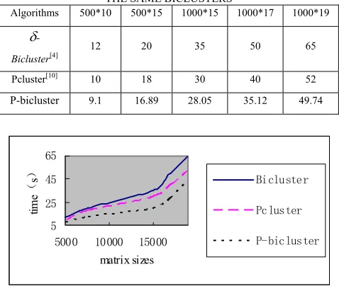
We first sequentially implement our algorithm and compare the performance with other two algorithms. In Pcluster and our algorithm, we set δ=6, the least number of rows Nr=5,the least number of columns Nc=30, and k=50. For a 500*10 matrix, our algorithm can find 50 biclusters in 9.1 seconds, while δ-Bicluster and Pcluster have to cost 12s and 10s to detect these 50 biclusters. For a 1000*17 matrix, our algorithm costs 35.12s, but δ -Bicluster costs 50s and Pcluster costs 40s. Table 1 and figure 2 show the comparison of the computational time of our algorithm with that of other algorithms for getting the same biclustering results.
TABLE Ⅰ.
COMPARISON OF THE COMPUTATIONAL TIME OF OUR ALGORITHM WITH THAT OF OTHER ALGORITHMS GETTING
THE SAME BICLUSTERS
Algorithms 500*10 500*15 1000*15 1000*17 1000*19
δ
-Bicluster[4] 12 20 35 50 65
Pcluster[10] 10 18 30 40 52
P-bicluster 9.1 16.89 28.05 35.12 49.74
5 25 45 65
5000 10000 15000 matrix sizes
tim
e
(s
) Bicluster
Pcluster
P-bicluster
Figure 2. Comparison of the computational time of our algorithm with that of other algorithms getting the same bicluster
From Table1 and figure 2 we can see that sequential implementation of our algorithm is obviously faster than other algorithms under the same condition.
0 10 20 30 40 50
1 3 5 7
number of processors
time
(s) 500*10
500*15 1000*15 1000*17 1000*19
Figure 3. Computational time of our algorithm using different processor numbers
We also test our parallel algorithm using the human gene expression data[17] on the massive parallel processors
Shenteng 1800 using MPI (C bounding). The computational time by using different numbers of processors are shown in figure.3. From figure.3 we can see that the computation speed will become faster as the number of processors increases. But the speedup will be decreased when the number of processors is larger than 7. Due to the overhead of communication between processors which increases the total time of the algorithm, the speedup of our algorithm can not increase linearly with the growth of processors exactly. This is in conformity with the Amdahl’s Law.
We also compare the quality of biclusters by our algorithm with that by several other algorithms. Figure. 4 shows a set of biclustering results obtained by our algorithm. In the figure, the wide line denotes the bicluster lost by algorithm Pcluster and the dot line denotes the bicluster lost by algorithm δ-Bicluster. From figure.4 we can see that our algorithm can find more biclusters and has higher biclustering quality than other similar methods.
-2000 -1000 0 1000 2000
0 10 20 30 40 50
conditions
expressing level
Figure 4. Biclusters get by our algorithm
VI.CONCLUSIONS AND FUTURE WORK
gradually adding columns and rows on the data sets. Experimental results show that our algorithm has superiority over other similar algorithms in terms of processing speedup and quality of clustering and efficiency.
ACKNOWLEDGMENT
This research was supported in part by the Chinese National Natural Science Foundation under grant No. 60673060, Natural Science Foundation of Jiangsu Province under contract BK2008075, and the Graduated Education Research Foundation of Jiangsu Province.
REFERENCES
[1] G. Getz, E. Levine, and E. Domany. Coupled two-way clustering analysis of gene microarray data. In Proceedings of the Natural Academy of Sciences USA, pages 12079– 12084, 2000.
[2] Chun Tang, Li Zhang, Idon Zhang, and Murali Ramanathan. Interrelated two-way clustering: an unsupervised approach for gene expression data analysis. In Proceedings of the 2nd IEEE International Symposium on Bioinformatics and Bioengineering, pages 41–48, 2001. INESC-ID TEC. REP. 1/2004, JAN 2004 31
[3] J. A. Hartigan. Direct clustering of a data matrix. Journal of the American Statistical Association (JASA), 67(337):123–129, 1972.
[4] Yizong Cheng and George M. Church. Biclustering of expression data[J]. In Proceedings of the 8th International Conference on Intelligent Systems for Molecular Biology
(ISMB’00), pages 93–103, 2000.
[5] Jiong Yang, Wei Wang, Haixun Wang, and Philip Yu. Æ-clusters: Capturing subspace correlation in a large data set. In Proceedings of the 18th IEEE International Conference on Data Engineering, pages 517–528, 2002
[6] Jiong Yang, Wei Wang, Haixun Wang, and Philip Yu. Enhanced biclustering on expression data[C]. In Proceedings of the 3rd IEEE Conference on Bioinformatics and Bioengineering, pages 321–327, 2003. [7] Yuval Klugar, Ronen Basri, Joseph T. Chang, and Mark
Gerstein. Spectral biclustering of microarray data: coclustering genes and conditions. In Genome Research, volume 13, pages 703–716, 2003.
[8] Amir Ben-Dor, Benny Chor, Richard Karp, and Zohar Yakhini. Discovering local structure in gene expression data: The order–preserving submatrix problem. In
Proceedings of the 6th International Conference on Computacional Biology (RECOMB’02), pages 49–57, 2002
[9] Zonghong Zhang, Alvin Teo. Mining Deterministic Biclusters in Gene Expression Data. In Proceedings of the Fourth IEEE Symposium on Bioinformatics and Bioengineering (BIBE’04), pages 2173-2180,2004
[10]Haixun Wang, Wei Wang, Jiong Yang, and Philip S. Yu. Clustering by pattern similarity in large data sets. In
Proceedings of the 2002 ACM SIGMOD International Conference on Management of Data, pages 394–405, 2002 [11]Sungroh Yoon, Giovanni De Micheli. An Application of
Zero-suppressed Binary Decision Diagrams to Clustering Analysis of DNA Microarray Data. In Proceedings of the 26th Annual International Conference of the IEEE EMBS.
2004, pages 2925-2928.
[12] Amos Tanay, Roded Sharan, and Ron Shamir. Discovering statistically significant biclusters in gene
expression data. In Bioinformatics, volume 18 (Suppl. 1), pages S136–S144, 2002
[13]Laura Lazzeroni and Art Owen. Plaid models for gene expression data. Technical report, Stanford University, 2000.
[14]Qizheng Sheng, Yves Moreau, and Bart De Moor. Biclustering micrarray data by gibbs sampling. In
Bioinformatics, volume 19 (Suppl. 2), pages ii196–ii205, 2003
[15]Eran Segal, Ben Taskar, Audrey Gasch, Nir Friedman, and Daphne Koller. Rich probabilistic models for gene expression. In Bioinformatics, volume 17 (Suppl. 1), pages S243–S252, 2001
[16]Eran Segal, Ben Taskar, Audrey Gasch, Nir Friedman, and Daphne Koller. Decomposing gene expression into cellular processes. In Proceedings of the Pacific Symposium on Biocomputing, volume 8, pages 89–100, 2003
[17] http://arep.med.harvard.edu/biclustering/
W. Liu was born in Jiangyin, Jiangsu Province, P.R.China, in July 1, 1982. She received B. Sc degree and M. Sc degree in computer science from Yangzhou University, P.R. China in 2004 and 2007 respectively. She is currently a Ph.D candidate in the Institute of Information Science and Technology, Nanjing University of Aeronautics and Astronautics, Nanjing, P.R.China.
Her research interest includes data mining, bioinformatics and parallel processing. She has published more than 10 papers in journals and conferences.
L. Chen was born in Baoying, Jiangsu Province, P.R.China, in September 10, 1951. He received B. Sc degree in mathematics from Yangzhou Teachers’ College, P.R. China in 1976.
He is currently professor of computer science, and the dean of Information Technology College, Yangzhou University, Jiangsu Province, P.R. China. He has published more than 120 papers in journals including IEEE Transactions on Parallel and Distributed System, Journal of Supercomputing, The Computer Journal. In addition, he has published over 100 papers in refereed conferences. He has also co-authored/co-edited 5 books (including proceedings) and contributed several book chapters. His research interest includes data mining, bioinformatics and parallel processing.