A New Methodology for Frequency Estimation of
Second or Higher Level Domino Accidents in
Chemical and Petrochemical Plants Using
Monte Carlo Simulation
Abdolhamidzadeh, Bahman; Rashtchian, Davood*+; Ashuri, Elham
Department of Chemical and Petroleum Engineering, Sharif University of Technology, Tehran, I.R. IRAN
ABSTRACT: Some of the most destructive accidents of 1980s and 90s which occurred in process industries were domino accidents. Although domino accidents are among the most destructive industrial accidents, there are not much pioneering works done on quantification of them. The analytical formulation of the domino accidents is usually complex and need a deep knowledge of probability rules. Even if the case is formulated, errors in calculation such as round-off error, is very probable as the values used all have small quantities and the number of possible scenarios are too high. In this paper, a new methodology based on Monte Carlo Simulation (MCS) technique is proposed for frequency estimation of domino accidents. The applicability and flexibility of this method is evaluated while applying it to estimate domino frequencies in a case study very similar to a real industrial plant. The simulation technique has shown advantages in comparison to analytical probability methods. The major advantage is non-dependency of the accuracy of results to complexity of the system. In addition by using simulation techniques, failure probability can be calculated as a function of time.
KEY WORDS: Domino accidents, Frequency estimation, Monte Carlo simulation, Chemical process safety.
INTRODUCTION
AIChE (American Institute of Chemical Engineers) defines domino effect as “an incident which starts in one item and may affect nearby items by thermal, blast or fragment impact, causing an increase in consequence severity or in failure frequencies” [1].
Lees defines a domino accident as “an event at one unit that causes a further event at another unit” [2] or Cozzani et al. states that “a domino accidental event will
be considered as an accident in which a primary event propagates to nearby equipment, triggering one or more secondary events resulting in overall consequences more severe than those of the primary event [3]”. Considering the different terms in the above definitions there are some common conditions. In almost all of the definitions, three accepted steps for a domino accidental scenario to occur are mentioned. A primary accidental scenario, which *To whom correspondence should be addressed.
+E-mail: [email protected]
initiates the domino sequence; a propagation of the primary event, due to an “escalation vector” generated by the physical effects of the primary scenario, that results in the damage of at least one secondary equipment item; and finally one or more secondary events (i.e. fire, explosion and toxic dispersion), involving the damaged equipment items. Another condition about domino accidents is that severity of the domino accident should be higher than that of the primary event taken place stand-alone.
Some of the most destructive accidents of 1980s and 90s which occurred in chemical process industries were domino accidents. Fire and explosion in HPCL refinery, Vishakhapatnam, India (1997) led to over 60 deaths and huge damage to property [4] or series of explosions in a LPG complex in Mexico City (1984) caused more than 500 deaths [5]. Even in Iran accidents such as Neyshabur train tragedy (2004) or a very recent series of fire and explosions in two adjacent chemical plants in Arak (2008) are representative of domino accidents [6].
Construction of chemical and petrochemical plants close to each other forming large industrial clusters is a common practice in many developing countries such as those in Middle East especially in Iran (e.g. Mahshahr and Assaluyeh). These complexes are in some cases located near densely populated residential areas. It is quite clear that hazard analysis of such process plants should not be confined to the occurrence of stand-alone incidents, but the possibility of domino occurrence should be considered as well. So assessment of risk caused by domino accidents in process plants should be considered as a necessary part of any quantitative risk analysis (QRA) study. Many analytical studies and experimental evidencesshowthat performing QRA without considering domino accidents leads to risk underestimation. In spite of the importance of such kind of accidents in process industries, a well assessed methodology for the quantitative estimation of the risk driven from these events is still not available. In risk assessment consequence and frequency of every accident should be considered simultaneously [1]. Each one requires its own methods to be estimated. The present study is focused on domino frequency estimation. There are some methods presented that are reviewed here in brief.
One way to deal with domino accidents is to increase occurrence frequency of identified major incidents for an equipment in a system comparing the case where it is
single to the case with the knock-on contribution. In fault tree terms, extra external events are added to account for domino mechanisms leading to the top event. This method was employed by HSE (1978) in performing a safety analysis and mentioned by CCPS (2000) as an acceptable method for QRA [1]. Another method is proposed by Bagster and Pitblado (1991) that works entirely in the frequency domain. They claimed that their method is capable of estimating the frequency of not only first level domino scenarios but also second level or more [8]. Their method was only capable of calculating probability of damage in a single unit due to accident in another unit. Bagster and Pitblado have not focused on combination of events that usually occur in complex layouts after an accident in a primary unit. Another point is that this method like many others ignores the time dependence of probabilities for frequency estimation. It is obvious that the probability of occurrence of many primary events have a time dependent distribution.
Khan and Abbasi (1998) in a paper on domino effect modeling proposed some specific methods for domino frequency estimation as a part of their DEA (Domino Effect Analysis) procedure [8]. They have applied the method to assess thedomino riskin some chemical plants. Cozzanietal.(2005)developed a systematic procedure for the quantitative assessment of the risk caused by domino effect. In their method a simplified technique was introduced for consequence and vulnerability assessment of domino scenarios. They also proposed a method to assess the frequency of these events [9]. Cozzani et al. have neglected the probability of escalation to second level or more in their procedure, so the method is valid for only first level scenarios. One of the advantages of the latter method is considering the combination of events and its ability to estimate probability for them.
big analytical formulas, round-off error will be significant and make the results erroneous.
ANALYTICAL FORMULATION OF EQUIPMENT FAILURE FREQUENCIES
Although analytical formulation of the domino cases is difficult, especially when the number of equipments in a system increases, it should be done for comparison with the results of the simulation in order to check the validity of the method which will be proposed further. So the objective in this part is to generate an exact formula based on probability distribution function that gives the instantaneous rate of failure of each component in system like process equipment in a chemical plant. All the pioneering methods neglected the time dependence of failure rates for process equipments for the sake of simplicity. But in this part of the paper it has been tried to develop an exact formulation of domino case taking into account time dependence.
The exponential distribution has been used to model the failure probability of the equipments in this study. It is a realistic assumption because many components during their useful lifetime exhibit a constant hazard rate. Such a rate implies that the occurrence of failures is purely random and that there is no deterioration of the strength or performance of the components with time. Although this assumption is not realistic for the whole lifetime of the equipment, it is a good approximation during its useful lifetime. A constant hazard rate is modeled by exponential distribution, a model that is simple, requires only one parameter to be defined, and is probably the most widely used distribution in reliability analysis. The failure rate of such equipment can be written as:
i
i(t)=λ
λ =constant (1) The constant failure rate of any equipment can be a generic data or can be calculated using Fault Tree or Event Tree methods. Using basic reliability formulas, reliability and unreliability of such an equipment can be expressed as follows:
P(no failure of component i in the time interval 0 to t)= Ri(t)= e it
λ −
(2) P(failure of component i in the time interval 0 to t)= Qi(t)= 1 e it
λ −
− (3)
It is obvious from the above equations that failure or survival is not expressed instantaneously but over a time period. The instantaneous failure probability using the memory-less nature of exponential distribution can be written as:
t
t i
i ).e
e 1 (
P= − −λ∆ −λ (4)
Where P is the probability of survival up to t, but occurrence of a failure in a time interval after t. This is the instantaneous failure probability for component i independent of other components or in isolation. But as described before, it is desired to have a formula giving the failure probability of any equipment not only by its failure but also due to effect of accident in other equipments (considering probability of domino accidents in a plant). Other equipments by causing escalation vectors such as radiation, overpressure or fragment projection may trigger an accident in equipment i. Probability of escalation of an accident which occurred in any equipment like j to i that can be estimated from credible methods such as Probit models for any accident, is called Pji here. Then the failure probability of component i due to component j failure is:
t t ji
no
domi j j
ji( t) P .(1 e ).e
P ∆ = − λ∆ −λ (5) So the total instantaneous failure probability of component i, if just one other equipment j exists is:
+ −
− −
=
∆t) (1 e−λ∆ ).e−λ (1 (P (1 e−λ∆ ).e−λ )
(
Pi i t it ji j t jt (6)
Pji(1 e j t).e jte it
λ − λ − ∆ λ −
−
For example for a three equipment case, i, j and k, the failure probability of component i will be:
)) e 1 ( P 1 ))( e 1 ( P 1 ( e ) e 1 ( ) t (
P ki t
t ji t t
i i i j k
λ − λ − λ − ∆ λ − − − − − − =
∆ (7)
)) e 1 ( P 1 ))( e 1 ( P 1 ( e e ) e 1 (
P kj t
t ki t t t
ji j i j k k
λ − λ − λ − λ − ∆ λ − − − − − − + )) e 1 ( P 1 ))( e 1 ( P 1 ( e e ) e 1 (
P jk t
t ji t t t
ki k i k j j
λ − λ − λ − λ − ∆ λ − − − − − − +
The above formula evaluates failure probability of component i in time interval t assuming its survival up to t. This can be generalized for any system with n independent components as:
∏
≠ = λ − λ − ∆ λ − − − − = ∆ n i j 1 j t ji t ti( t) (1 e )e (1 P (1 e ))
P i i j (8)
∏
≠ = ≠ = ∆ λ − λ − λ − ∆ λ − − − × − + n i k 1 k n k , i l 1 l t li t t tki(1 e )e e [(1 P (1 e ))
P k i k l
))] e 1 ( P 1
( − lk − −λl∆t
It is quite obvious that the mathematical formulation of the equipment failure frequency is complex and need a deep knowledge of probability rules. Even if the case is formulated, errors in calculation such as round-off error is very probable as the values used all have small quantities. Due to the complexity and limitations of exact analytical formulations, an alternative method is proposed that overcomes the disadvantages and shortcomings of analytical solution. This method is based on using simulation techniques.
SIMULATION TECHNIQUES
Insystem reliability analysis and frequency estimation
there are some alternative methods generally designated as simulation techniques. In these simulation techniques analytical solution and complex mathematical operations are not required. So it seems that simulation techniques for complex systems are more practically feasible.
One of the simulation techniques which have had a great impact in many different fields of computational science is a technique called Monte Carlo Simulation (MCS). MCS uses random numbers to model a process and then it is possible to evaluate factors such as process outcome frequencies. The process outcome can be defined differently for different applications. For example failure of an equipment can be a process outcome. This
technique works particularly well when the process is one where the underlying probabilities are known but the results are more difficult to determine. This method simulates systems with more than one uncertain input parameter with high accuracy [11, 12]. In domino frequency analysis, probabilities of primary event with all the escalation parameters are uncertain input parameters.
There are both advantages and disadvantages using MCS in comparison with analytical modeling [13]:
- The solution time for analytical techniques is relatively short, whereas usually extensive for simulation techniques. The extensive time is the result of iterative nature of this method. This is becoming less of a problem with today modern computers.
- Simulation techniques can provide a wide range of
output parameters including different probability
functions, but analytical methods are usually limited only to expected values.
- The model used in analytical techniques is usually a simplification, especially for complex systems or combinations. The MCS method is independent of how complex the system is.
- MCS is often criticized as being an approximate technique. However, in theory at least, any required level of precision can be achieved by simply increasing the number of iterations in a simulation. The limitation is then usually about the required CPU time.
USING MONTE CARLO SIMULATION IN DOMINOACCIDENT FREQUENCY ESTIMATION
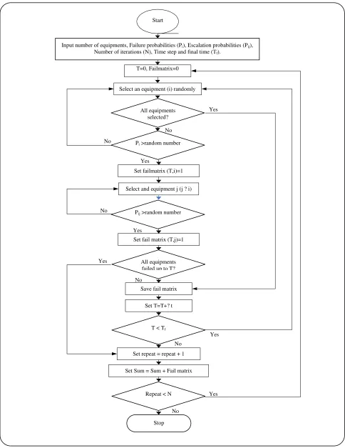
Due to the capabilities of Monte Carlo method that was mentioned before, it is used to estimate the failure probability of equipments both in isolation and in domino cases. The logic of the Monte Carlo algorithm for calculating the instantaneous failure probability of each equipment is outlined in Fig. 1.
At the first stage (initialization), the desired values for
the number of equipments (n), failure rates ( i) for any
equipment in isolation, escalation probabilities (Pij), number of iterations (N), time step ( t) and the final time
(tfinal) are specified. Also a matrix, named Failmatrix,
Fig. 1: Monte Carlo algorithm for calculating the instantaneous failure probability of equipments. T=0, Failmatrix=0
Select an equipment (i) randomly
Select and equipment j (j ? i) Set failmatrix (T,i)=1
Save fail matrix Set fail matrix (T,j)=1
Set T=T+? t
Set repeat = repeat + 1
Set Sum = Sum + Fail matrix Start
Input number of equipments, Failure probabilities (Pi), Escalation probabilities (Pij),
Number of iterations (N), Time step and final time (Tf).
All equipments selected?
Pi >random number
Pij >random number
All equipments failed up to T?
T < Tf
Repeat < N
Stop No
Yes No
Yes Yes
No Yes No
Yes No
No
calculated and compared with a generated random number (r1), in case that Ppe> r1 it means that this component fails at the time step, its related position in
Failmatrix is changed to one. It is assumed here that in
each t just one component can fail for the sake of
simplicity. In the innermost loop component j is checked whether it can cause domino effect, i.e. for each component (k) if Pjk is greater than a generated random number (r2) domino can occur (based on the concept of
MCS) and therefore its position in Failmatrix is changed
to one. These steps are repeated N times to compensate
for the stochastic nature of MC algorithm. For random
number generation, used in two steps of the algorithm, a
predefined function in MATLAB© software has been
used. Random numbers are a set of variables having values uniformly distributed between 0 and 1. There are different algorithms to generate random numbers. It is very important to select an algorithm which generates unbiased numbers.
The proposed procedure is easy to code, but there are some delicate points that should be considered. It is obvious that a component in each run can fail only once, so this condition should be checked each time when a component is set to fail by the algorithm. By this point at any time that all components are proved to have failed up to this time, the time loop is broken and a new iteration is started. By this method the run time of the program would be reduced greatly. Another point is that, it is not
necessary to save Failmatrix for any iteration. It is
sufficient that a new matrix is defined to save the
summation of the new Failmatrix with its previous values
in the past iterations, and finally the desired Failmatrix is
the last Failmatrix divided by N. In this way CPU time is
saved even with the highly iterative nature of this algorithm.
It should be mentioned that the proposed algorithm can be extended to estimate the failure frequency of equipments in second or higher levels domino accidents. This extension can be easily performed by adding another inner-loop to the algorithm. But as the probability of the second level domino accident is very low, it has been neglected in this study.
CASE STUDY
The proposed procedure is applied for analysis of a case study and comparing the result of simulation with
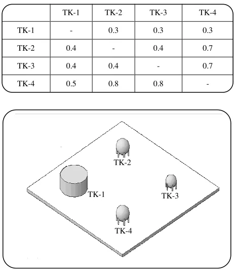
Table 1: Domino escalationprobability matrix used in the case
study.
TK-1 TK-2 TK-3 TK-4
TK-1 - 0.3 0.3 0.3
TK-2 0.4 - 0.4 0.7
TK-3 0.4 0.4 - 0.7
TK-4 0.5 0.8 0.8 -
Fig. 2: Sample layout selected as a case study.
exact mathematical solutions to show the validity of the procedure. The selected case is a hypothetical plant which is simulated with reference to the actual layouts of existing industrial plants. For the sake of simplicity, in general a single fail scenario is associated with any equipment and considered as the only possible primary and/or secondary event which can occur. There are four equipments present in the case, an atmospheric storage tank TK-1 (a crude oil floating roof storage tank) and three pressurized spherical tanks TK-2-4 (containing LPG). The layout is shown in Fig. 2.
The failure frequency for TK-1 to TK-4 in isolation are assumed 0.01, 0.09, 0.09, and 0.07 respectively. These failure rates are determined with reference to
technical documentsandwith considering each equipment
safeguards. The escalation probabilities defined as Pij in this study for the equipments are tabulated in table 1. Escalation probability is the probability that an accident in equipment i triggers a cascading accident in equipment j. (It should be noted that in this study calculation of primary event frequency or escalation probability is not the goal, there are methods such as Event Tree Analysis or Probit models to calculate those data which are utilized
TK-2
TK-1 TK-3
Fig. 3: Simulated and analytical instantaneous failure probability of isolated component 2 Vs. time ( t=0.5 year).
in the pioneering studies. The main goal in this study is evaluating the new method to estimate the failure frequency of equipments in complex systems especially for combinations of accidents for witch analytical solutions are not easily applicable.)
It is clear that P1j is less than other Pij’s (i j) as TK-1 is an atmospheric tank. For applying the stochastic simulation algorithm for the case study, at first a single tank is considered.
RESULTS AND DISCUSSION
Fig. 3 shows the instantaneous failure probability of TK-2 versus time without considering possibility of domino effect from other components. For this case t has been selected equal to 0.5 year. The result of analytical solution is compared with the results of simulation. The results of analytical solution are shown with a solid line in the figure and those of simulation with dots.
In the above two figures Equation (4) has been used for analytical solution. In Fig. 4, the instantaneous failure
probability of isolated TK-1 ( 1=0.01) is compared with
isolated TK-2 ( 2=0.09). But as 2 has a small value, t
has been considered one year to have lower iterations in the algorithm. It is obvious in Fig. 4 that the failure rate of component 1 is much lower than component 2. It can be seen that the results of MC algorithm can accurately predict the analytical equation.
In the next step of checking the algorithm, two tanks from the case study are considered (TK-1 and 2) to have mutual effects. In this case Equation-6 was used for
Fig. 4: Simulated and analytical instantaneous failure probability of isolated component 1 and isolated component 2 vs. time ( t=1.0 year).
analytical results. As it was expected, because of the low failure rate of TK-1, the instantaneous failure probability of isolated TK-2, which was shown in Fig. 3, is just a little lower than this failure probability of TK-2 in the vicinity of component 1, in Fig. 5.
Finally the algorithm is used for the analyzing the whole system of the case study (system consisting of four tanks) and comparing the results with that of analytical equation. This comparison is demonstrated in Fig. 6. It is clear that the overall performance of the algorithm is acceptable. The comparison of the instantaneous failure probability of isolated TK-2 (Fig. 3) with the case, in which this tank can have mutual effects with three other components, shows how domino effect can increase the failure probability of each tank.
Figs. 3-6 offer convincing proof of the feasibility of the stochastic simulation algorithm for system reliability estimation and the advantage of their usage instead of complicated derived analytical equations. It should be noted that writing an analytical relation to obtain the failure frequency of an equipment is not always feasible. In real industrial cases with a high number of equipments having mutual effect, it is not simple to derive an analytical formulation to determine the failure frequency. So analytical formulation is good only for simple cases or comparison and checking proposed simulation techniques like the one in this paper.
CONCLUSIONS
This paper highlights the difficulties in analytical
domino accident frequency estimation. Some of the 0 5 10 15 20 25 30 35 40 45 50
Time (year)
0 10 20 30 40 50 60 70 80 90
Time (year) 0.09
0.08 0.07 0.06
0.05
0.04 0.03 0.02
0.01 0
In
st
a
n
ta
n
eo
u
s
fa
il
u
re
p
ro
b
a
b
il
it
y
Monte carlo simulation for component 2 Analytical solution for component 2 Monte carlo simulation for component 1 Analytical solution for component 1 Monte carlo simulation (n=1)
Analytical solution (n=1)
0.045 0.04
0.035
0.03 0.025 0.02
0.015
0.01
0.005
0
In
st
a
n
ta
n
eo
u
s
fa
il
u
re
p
ro
b
a
b
il
it
y
o
f
co
m
p
o
n
en
t
Fig. 5: Simulated and analytical instantaneous failure probability of component 2 considering domino effect of component 1 vs. time ( t=0.5 year).
existing methods are reviewed and their advantages and shortcomings are described. In this paper due to the capabilities and advantages of using simulation techniques, Monte Carlo Simulation (MCS) has been used to estimate the failure frequency of process equipments in domino accidents. The algorithm used in this way is explained. For the validation of the proposed method, the results of the simulation have been compared with the exact analytical solution in a case very similar to a real process plant. Different possible scenarios have been defined and simulated.
There was excellent agreement between the analytical and simulation output. But the simulation technique has
shown advantagesin comparison with analytical methods.
The major advantage is non-dependency of the results accuracy to complexity of the system. Another advantage when using MCS is time dependency of the primary event occurrence. None of the existing methods consider the time dependency because it makes the case too difficult to be modeled and solved analytically.
Received : 29th June 2008 ; Accepted : 3rd February 2009
REFERENCES
[1] CCPS, “Guidelines for Chemical Process Quantitative
Risk Analysis”, 2nd Ed., AIChE, New York (2000).
[2] Lees, F.P., “Loss Prevention in the Process
Industries”, 2nd Ed., Butterworths (1996).
[3] Cozzani, V. and Salzano, E., Threshold Values for Domino Effects Caused by Blast Wave Interaction
with Process Equipment, Journal of Loss Prevention
in the Process Industries, 17, p. 437 (2004).
Fig. 6: Simulated and analytical instantaneous failure probability of component 2 considering domino effect of other three components Vs. time ( t=0.5 year).
[4] Khan, F.I. and Abbasi, S.A., DOMIFFECT (DOMIno
eFFECT):User-FriendlySoftwarefor Domino Effect
Analysis, Environmental Modeling & Software,
13, p. 163 (1998).
[5] Pietersen, C. M., Analysis of the LPG Disaster in
Mexico City, Loss Prevention and Safety Promotion,
5, p. 21 (1986).
[6] UNEP APELL - Awareness and Preparedness for Emergencies on a Local Level: www.uneptie.org [7] Bagster, D.F. and Pitblado, R.M., The Estimation
of Domino Incident Frequencies - An Approach,
Trans. IChemE, 69, Part B (1991).
[8] Khan, F.I. and Abbasi, S.A., Models for Domino Effect Analysis in Chemical Process Industries,
Process safety Progress, 17 (1998).
[9] Cozzani, V., Gubinelli, G., Antonioni, G., Spadoni, G. and Zanelli, S., The Assessment of Risk Caused by Domino Effect in Quantitative Area Risk Analysis,
Journal of Hazardous Materials, A127, p.14 (2005). [10] Rashtchian, D. and Lak, A., Risk Assessment of
Ammonia Storage Tanks, NSMSI, 26(4), (2007).
[11] Billinton, R. and Allan, R., “Reliability Evaluation of Engineering Systems: Concepts and Techniques”,
2nd Ed., Plenum Press (1992).
[12] Vose, D., “Risk Analysis: A Quantitative Guide”,
2nd Ed., John Willey & Sons (2000).
[13] U.S. Environmental Protection Agency, “Guiding Principles for Monte Carlo Analysis”, EPA/630/R-97/001 (1997).
0 5 10 15 20 25 30 35 40
Time (year) 0 10 20 30 40 50 60 70 80 90
Time (year)
0.1 0.09 0.08
0.07 0.06 0.05 0.04
0.03 0.02 0.01
0
In
st
a
n
ta
n
eo
u
s
fa
il
u
re
p
ro
b
a
b
il
it
y
o
f
co
m
p
o
n
en
t
2
0.09 0.08
0.07 0.06
0.05
0.04
0.03
0.02 0.01
0
Monte carlo simulation for component 2 Analytical solution for component 2 Monte carlo simulation for component 1 Analytical solution for component 1