EXPLORING THE STATISTICAL RELATION BETWEEN THE
UNDERWATER ACOUSTIC AND OPTICAL CHANNELS
Roee Diamanta, Filippo Campagnarob, Michele De Filippo de Graziac, Alberto Testolinc, Violeta Sanjuan Calzadod, Michele Zorzib, Paolo Casarie
a Department of Marine Technology, University of Haifa, Israel b Department of Information Engineering, University of Padova, Italy c Department of General Psychology, University of Padova, Italy
d NATO STO Centre for Maritime Research and Experimentation, La Spezia, Italy e IMDEA Networks Institute, Madrid, Spain
Contact author: Roee Diamant, The Leon H. Charney School of Marine Sciences, Room 280, Multi Purpose Building, University of Haifa, 199 Aba Khoushy Ave., Mount Carmel, Haifa 3498838, Israel. Phone: +972-4-8288790. Fax : +972-4-8288267
Abstract: In this paper, we are interested in finding whether a statistical relationship exists between underwater acoustics and optics, despite the different physics that govern these technologies. Besides the theoretical interest of such a relationship, predicting the quality of the optical links through acoustics is relevant for multimodal communications.
Our study is based on a large dataset acquired during the NATO ALOMEX 2015 expedition. The dataset consists of several acoustic and optical link characteristics measured at multi-ple locations, reflecting a diversity of sea environments. Our results, based on a systematic machine learning analysis, show a strong correlation between the properties of acoustic links and the reliability of optical communications. Potentially, this can be leveraged to predict the state of underwater optical links.
Keywords: Underwater acoustic communications; Underwater optical communications; Multimodal systems; Machine learning; Sea Experiment.
INTRODUCTION
characterized by long-range (in the order of tens of km) but low-data-rate transmissions (up to a few kbps), and is considered highly unreliable due to the limited bandwidth, long delay spread, short channel coherence time, and dispersiveness that characterize the acoustic chan-nel [1]. OC features high data rates (in the order of Mbps), but is only suitable over much shorter transmission ranges (practically up to tens of meters).
AC and OC are driven by different physics. The former involves the propagation of a pressure wave and is modelled, e.g., via the so-called normal modes or empirical equa-tions [2], whereas the latter is performed via electromagnetic waves whose propagation is driven by the radiative transfer equations [3]. The sources of noise in the underwater acous-tic channel are also much different than those that affect the opacous-tical channel. For example, the irradiance and scattering of sunlight in the water are the main factors that affect OC. Although AC and OC are seemingly unrelated, it is of theoretical interest to show if there exists a combination of underwater acoustic properties that can be exploited to predict the state of underwater optical links at a given range and depth.
While finding a relation between the AC and OC is of theoretical interest per se, such relation also has several practical applications. Predicting the characteristics of OC through AC, would help, e.g., guide a mobile node which holds both communication systems to a location where OC can be efficiently used. This application is specifically important for multi-modal underwater communication systems, where both OC and AC are utilized [4]. Moreover, exploiting a relationship between OC and AC would enable more effective switching mechanisms.
In this work, we study the relationship between AC and OC from a statistical point of view in environments such as the open sea, where it can be assumed that the properties of optical links change slowly over time and space. Our work does not include a theoretical explanation of the mutual relation between AC and OC, but rather is limited to showing that such a relation exists, with the hope to stimulate further theoretical investigations.
Our study is based on a large dataset of acoustic and optical link properties simultane-ously measured over a prolonged time span and over different frequency bands. The dataset was obtained during the ALOMEX 2015 experiment led by the NATO STO CMRE, La Spezia, Italy. Using this dataset, we trained different learning models using support vector machines (SVMs) [5], with the goal of classifying the corresponding quality of the optical link at various distances and depths. The system was designed to maximize accuracy, while avoiding overfitting.
Our results show a strong correlation between the properties of ACs and the overall qual-ity of the OC, with a sufficient degree of accuracy to enable mechanisms that intelligently switch between acoustic and optical underwater communication technologies, as well as to evaluate the radiance properties of the water.
BACKGROUND
AC is also highly affected by the channel ambient noise, usually modelled as an isotropic coloured Gaussian process whose power spectral density reduces by 10 dB per octave [6]. However, the acoustic ambient noise may also include location-dependent, non-isotropic noise, whose time-varying characteristics also affect the performance of AC. The SNR (in dB) of a transmission performed at a frequency 𝑓𝑎 over a distance 𝑑 between the trans-mitter and the receiver is empirically modelled as:
𝑆𝑁𝑅(𝑑, 𝑓𝑎) = 10 log10(𝑁(𝑓𝑃𝑎
𝑎) 𝛿𝑓𝑎) − 𝐴(𝑑, 𝑓𝑎) (1)
where 𝑃𝑎 is the source level (usually expressed in dB relative to 1 𝜇Pa @ 1 m from the source), 𝑁(𝑓𝑎) is the noise level, 𝐴(𝑑, 𝑓𝑎) is the power attenuation in dB, and 𝛿𝑓𝑎 is a narrow band around 𝑓𝑎 where we can assume 𝐴(𝑑, 𝑓) = 𝐴(𝑑, 𝑓𝑎) and 𝑁(𝑓) = 𝑁(𝑓𝑎).
Optical communications basics ―Light traveling in the water interacts with the particu-lates and dissolved materials within the water as well as the water molecules themselves. These interactions produce light attenuation (modelled via an attenuation rate per unit length travelled by the wave, termed 𝑐) that will determine the underwater light field, or radiance, denoted as 𝐿, and defined as the measure of light energy leaving an extended source in a particular direction.
The parameters 𝐿 and 𝑐 are related through the radiative transfer equation (RTE), which relates the apparent and inherent optical properties of the medium [3]. The light attenuation rate 𝑐, the optical absorption rate 𝑎, and the loss rate due to scattering processes 𝑏 are related as 𝑐 = 𝑎 + 𝑏. If the inherent optical properties of the medium depend only on depth, inelas-tic processes are ignored, and there are no internal sources, the time-dependent RTE is de-scribed as [7]
cos 𝜃𝑑𝐿(𝑧,𝜆,𝜃,𝜑)𝑑𝑧 = −𝑐(𝑧, 𝜆)𝐿(𝑧, 𝜆, 𝜃, 𝜑) + ∫ 𝛽(𝑧, 𝜆, 𝜃′, 𝜑′→ 𝜃, 𝜑)𝐿(𝑧, 𝜆, 𝜃′, 𝜑′)𝑑𝛺′
4𝜋 ,(2)
where 𝛽(∙) is the volume scattering function, which describes how the medium scatters light per unit length and solid angle. The polar angle 𝜃 and the azimuthal angle 𝜑 of a spherical coordinate system specify the scattered light direction, whereas the coordinates (𝜃′, 𝜑′) convey the direction of the incident light. The integration is performed over the unit sphere surface, and we recall that 𝑑𝛺′= sin 𝜃′𝑑𝜃′𝑑𝜑′. At a given depth and wavelength, 𝐿 is usually referred to as the radiance distribution. The first term on the right hand side of (2) represents the loss of radiance along (𝜃, 𝜑), while the second term provides the gain in radiance from all other directions. Analytical solutions of the RTE (2) are possible only if scattering is negligible. Otherwise, as in the present work, (2) must be solved numerically, e.g., see [7].
For this study, we are interested in the scalar irradiance 𝐸0, measured over all directions, obtained by integrating radiance over the whole sphere as
𝐸0(𝑧, 𝜆) = ∫ 𝐿(𝑧, 𝜆, 𝜃, 𝜑)𝑑𝛺4𝜋 . (3)
In the case of light transmission for underwater optical communications, this will be affected by the ambient light, considered as noise and computed as 𝑁𝐴 = (𝑆 ∙ 𝐸0∙ 𝐴𝑟)2, where 𝑆 and
𝐴𝑟 are the receiver’s sensitivity and area, respectively.
In particular, we use an efficient class of learning algorithms called support vector ma-chines (SVMs) [5]. An SVM tries to achieve the best separation between patterns belonging to different classes by finding the maximum-separation hyperplane that has the largest dis-tance to the nearest training data point of any class. As a result, this learning framework is particularly indicated when the available data is limited. A similar framework can be applied in the case of real-valued outputs (regression tasks) using a variant called Support Vector Regression (SVR) [8].
We consider both linear and non-linear SVMs. In linear SVMs, we assume that the pat-terns are linearly separable. The equation of a linear SVM is expressed in the form
𝑓(𝑥) = ⟨𝑤⃗⃗ , 𝑥 ⟩ + 𝑏 , (4)
where ⟨∙,∙⟩ denotes the inner product in ℝ𝑛, and the vector 𝑤⃗⃗ and scalar 𝑏 are used to define the position of the maximum-margin separating hyperplane. Geometrically, the distance be-tween the two external hyperplanes is 2/|𝑤⃗⃗ |, so we want to minimize |𝑤⃗⃗ | such that each data point lies on the correct side of the margin. The SVM training procedure amounts to solving a convex quadratic problem. The solution is a unique globally optimum result, for which
𝑤⃗⃗ = ∑𝑁𝑖=1𝛼𝑖𝑦𝑖𝑥 𝑖 . (5)
The terms 𝑥 𝑖 are called support vectors. Once an SVM has been trained, the decision func-tion can simply be written as
𝑓(𝑥 ) =sign(∑𝑁𝑖=1𝛼𝑖𝑦𝑖(⟨𝑥 , 𝑥 𝑖⟩) + 𝑏) . (6) The non-linear SVM uses the so-called kernel trick, implicitly mapping the inputs into higher-dimensional feature spaces. The resulting algorithm is formally similar to that of a linear SVM, except that every dot product is replaced by a non-linear kernel function
𝐾(𝑥 , 𝑥 𝑖). This allows the algorithm to fit the maximum-margin hyperplane in a transformed feature space. In this work we use the popular Gaussian Radial Basis Function (RBF) kernel:
𝐾(𝑥 , 𝑥 𝑖) = exp(−|𝑥 − 𝑥 𝑖|2/(2𝜎2)) . (7)
DESCRIPTION OF THE ACQUIRED DATASET
To validate our system we used a data set collected during the NATO ALOMEX 2015 mission. The experiment spanned 13 days across 2800 km from Southern Spain to West Africa. During this expedition, we measured both acoustic and optical link properties in the nine different stations marked in Fig. 1. Some stations were sampled in the same locations but at different times. In each station, a data collection lasting over an hour took place. The locations noted in Fig. 1 were chosen to represent different channel conditions. Stations 1-4 were located in the Mediterranean Sea, while Stations 5-9 were sampled in the Atlantic Ocean.
# LF band HF band
1 Noise level
2 RSSI
3 Delay spread
4 RMS channel tap amplitude
5 Number of channel taps
6 SNR Integrity
7 Channel length 8 Noise coherence time 9 Channel coherence time
Table I: List of measured acoustic channel erties in the LF band and HF bands. Blue prop-erties are common to both bands.
Fig. 1. Location of the measurement sites during the ALOMEX 2015 cruise.
provided by EvoLogics modems. This allowed us to estimate 9 different properties for LF channels and 6 for HF channels, as listed in Table I. Since the optical data was used as labeling for training and testing only, no pre-processing was performed. In the context of multimodal systems, we focused only on classifying and predicting the optical SNR during both nighttime and daytime. However, the same procedure can be carried out for other op-tical properties, such as the scattering or the total attenuation coefficients.
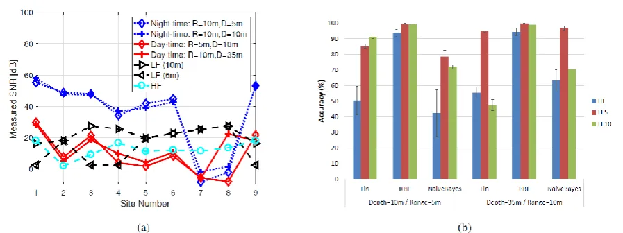
The OC dataset was used to train the SVM for classification purposes. For classification, the training procedure involved a threshold to label the trained OC dataset as “good” or “bad,” where the threshold (15 dB and 10 dB for daytime and nighttime measurements, respectively) is chosen so that “good” and “bad” training links occur more or less the same number of times, to avoid overfitting. In Fig. 2a, we show the SNR of the measured OC links during daytime and nighttime. The values shown lead to a variation of roughly 70 dB in the range of SNR. Naturally, this produces a large change in the number of “good” and “bad” OC channels. More specifically, the choice of these threshold levels yielded a “good” to “bad” channel ratio of about 60%.
Fig. 2. (a) Average values for the optical and acoustic SNR at different sites. Results show a range of roughly 70~dB during nighttime, and 40~dB during daytime for optical SNR. (b) Classification accu-racy for daytime OC, obtained using linear SVM and RBF SVM. Results suggest a clear non-linear relationship between acoustic properties (mostly LF5) and OC.
RESULTS
The classification accuracy for the test sets is reported in Fig. 2b for both the linear SVM and the non-linear SVM with the RBF kernel. We explore classification using all three types of acoustic measurements. In all cases, the marked difference between the linear SVM and the RBF kernel suggests that the relation between the acoustic properties and the optical link quality is non-linear. In order to better assess the robustness of the findings, as a control simulation we also performed the same classification task using a Naïve Bayes classifier [9]. The average accuracy obtained using this algorithm was closely aligned with that obtained with the linear SVM. For this reason, in the following discussion we drop the comparison with the Naïve Bayes classifier and only consider the SVM models.
The results indicate that the LF measurements provide a more accurate prediction of the quality of the optical link, approaching 100% of classification accuracy for the non-linear SVM. The LF measurements yield a much higher accuracy also for the linear SVM, except for the 35-m depth, 10-m range condition, where the performance of LF10 is similar to that obtained using HF.
The classification accuracy for the test sets to predict the optical SNR during nighttime is reported in Fig. 3. Also in this case, the non-linear kernel clearly outperforms the linear SVM, achieving about 100% classification accuracy in all conditions. In fact, for many dis-tance-depth pairs considered in Fig. 3, the performance of the linear SVM in is close to chance level (50%).
Similar to the case of daytime optical transmission, in the nighttime scenario the LF measurements (LF5 in particular) are better predictors for the quality of the optical link. However, when using the linear SVM, HF sometimes still outperforms LF10, especially for the conditions corresponding to long distances (20-m range). This suggests that, in nighttime conditions, the HF signal can be more reliable than in daytime conditions, ap-proaching a prediction accuracy of 100% for the non-linear SVM and of 80% for the linear SVM at long ranges.
Fig. 3. Nighttime optical SNR classification accuracy results, suggesting a clear non-linear relation between AC and OC properties.
properties and the OC quality. This relation seems to be non-linear, as the greatest accuracy is achieved by the SVM using the RBF kernel.
In order to better evaluate the classifier performance across different conditions, three additional performance measures were also computed from confusion matrices [45]: preci-sion (i.e., class agreement of the data labels with the positive labels given by the classifier), recall (i.e., effectiveness of the classifier to identify positive labels), and specificity (i.e., effectiveness of the classifier to identify negative labels). The complete results are reported in Table II. We observe that the obtained values for precision, recall and specificity are consistent across different acoustic datasets and environmental conditions, and are fully aligned with the accuracy results reported in Fig. 2 and Fig. 3. In particular, results show that indeed the non-linear classifier achieves much better performance on all metrics, and has no biases for any particular class.
Interestingly, the data seem to suggest that linear classification using LF measurements improves close to the surface. This needs to be investigated further, as not all collected data show this same trend, and we have no further evidence to prove it. However, we still con-jecture that linear classification might be in fact more precise near the surface. A possible explanation can be a high concentration of biological particles such as plankton in the upper water layer, which would scatter the acoustic wave and, during daytime, also sunlight. The collection of additional data in this specific scenario would be a necessary step to verify this conjecture.
CONCLUSIONS
Table II. Precision, recall and specificity values for all classification tasks.
ACKNOWLEDGMENTS
This work was supported by the EKOE (Environmental Knowledge and Operation Ef-fectiveness) program of the NATO STO Centre for Maritime Research and Experimentation (CMRE). The acoustic dataset was acquired with instruments from the anti-submarine war-fare (ASW) program of CMRE. We would like to thank the captain and the crew of NRV Alliance for their assistance during data collection at sea.
REFERENCES
[1] X. Lurton, An introduction to underwater acoustics - Principles and applications. Springer, 2002.
[2] F. Jensen, et al., Computational Ocean Acoustics, Springer-Verlag, 2000.
[3] R. Spinrad, K. Carder, and M. J. Perry, Ocean Optics. Oxford Monographs on Geology and Geophysics. Oxford University Press, USA, 1994.
[4] F. Campagnaro et al., “Implementation of a multimodal acoustic-optic underwater
net-work protocol stack,” in Proc. MTS/IEEE OCEANS, Shanghai, China, 2016.
[5] C. Cortes and V. Vapnik, “Support-vector networks,” Machine learning, vol. 20, no. 3, pp. 273–297, 1995.
[6] J. Hovem, Marine Acoustics. Peninsula Publishing, 2012.
[7] C.Mobley, Light and water: radiative transfer in natural waters. Academic Press,1994. [8] A. J. Smola and B. Schölkopf, “A tutorial on support vector regression,” Statistics and
computing, vol. 14, no. 3, pp. 199–222, 2004.
[9] J. Huang, J. Lu, and C. X. Ling, “Comparing Naive Bayes, Decision Trees, and SVM with AUC and Accuracy,” in Proc. IEEE ICDM, Melbourne, FL, Nov. 2003.