Article
1
Using a Counting Process Method to Impute
2
Censored Follow-up Time Data
3
Jimmy T. Efird1,*, Charulata Jindal1
4
1 Centre for Clinical Epidemiology and Biostatistics (CCEB), School of Medicine and Public Health, The
5
University of Newcastle (UoN), Australia; [email protected] (C. J.)
6
* Correspondence: [email protected]; Tel.: +1.650.248.8282
7
8
Abstract: Censoring occurs when complete follow-up time information is unavailable for patients
9
enrolled in a clinical study. The process is considered to be informative (nonignorable) if the
10
likelihood function for the censoring model cannot be partitioned into a set of response parameters
11
that are independent of the censoring parameters. In such cases, estimated survival time
12
probabilities may be biased, prompting the need for special statistical methods to remedy the
13
situation. The problem is especially salient when censoring is skewed toward the early phase of a
14
study. In this paper, we describe a method to impute censored follow-up times using a counting
15
process method.
16
17
Keywords: counting process; censoring; Cox proportional-hazard regression; Kaplan-Meier;
18
imputation; survival analysis
19
20
1. Introduction
21
Ideally, censoring in a survival analysis should be non-informative and not related to any aspect
22
of the study that could bias results [1-7]. For example, toxic side effects of an investigational drug
23
may prompt the most ill patients to withdraw early from the study. Other patients may opt to leave
24
before the intended end of a trial if the treatment is effective and they feel well. Even when censoring
25
is non-informative (e.g., relocation to another city because of plant closure), by chance alone, it may
26
still have a serious effect on estimated survival probabilities, especially if the dropouts occur early in
27
the study.
28
In this paper, we present an example of early censoring to illustrate how the resulting survival
29
probabilities may be biased. We then describe a method to impute censored follow-up times by
30
rearranging the data as a counting process and generating jump-point plots.
31
2. Materials and Methods
32
2.1 Imputing Censored Follow-up Times
33
Let denote the follow-up time for the ordered observation, given a total of
34
observations and integer valued time points
35
= + 1, = + 1, … , = + 1; ≥ . (1)
Accordingly,
36
≤ … ≤ (2)
and
37
2 Then,
38
∀ ∧ ∋: = 1 , = 1 , (4)
the counting process “indicator” variable assumes the value 0 if ≤ and corresponds
39
to a censored follow-up time (i.e., the outcome event, such as death, has yet to occurred by time ).
40
Otherwise, when the observation denotes an event, assumes the value 0 if < and the
41
value 1 if ≥ [8].
42
Next, we fit a multiple logistic regression model with + 1 covariates to the above counting
43
process data, i.e.,
44
= 1| , , , … = 1
1 + ⋯ (5)
where the first covariate denotes time and the remaining covariates , ,… ,
45
represent outcome related risk factors. Note that the selection of this model is arbitrary and any other
46
binary predictor equation could be substituted at this step. For example, the addition of a higher
47
order term to the model or taking the logarithm of a covariate might be desirable. Other possible
48
options include using a log-binomial or negative-binomial equation to model the data [9-10]. Model
49
fit may be assessed by examining diagnostic leverage and residual plots, in lieu of standard goodness
50
of fit tests, which would assume that the underlying counting process data are independently
51
distributed [11-13].
52
A jump-point plot for a particular covariate pattern corresponding to a censored follow-up time
53
may be obtained by plotting the model predicted values ̂ against the time variable . Let
54
denote the value of that maps to ̂ = .50 (i.e., maximum likelihood estimate of the mean
55
jump-point observation). The imputed censored follow-up time is given as
56
imp = , , , (6)
where is the natural upper limit for a patient’s follow-up time. For example, in the case of
57
cancer therapy, the maximum life expectancy of a patient rarely exceeds 101 years of age. For a patient
58
aged 89 at diagnosis, we see that is computed as 101 − 89 . The original censored follow-up
59
times are then replaced with imp . However, it is important to note that these follow-up times are
60
still treated as censored values rather than events when computing survival probability estimates.
61
Assuming Martingale independence and considering the event times to be binomially
62
distributed [i.e., the probability of an event occurring in a particular risk set is equal
63
to its expectation divided by the risk set size (accounting for censored and event times),
64
with corresponding variance equal to 1 − ], it follows that the resulting data be may
65
analyzed using standard methods for handling censored time-to-event observations (e.g.,
Kaplan-66
Meier and Cox proportional-hazards models) [14-15]. Here, the sampling variability for estimating
67
the imputed censored follow-up times is absorbed into the sampling variability for each binomially
68
distributed event time, given that the estimates are asymptotically consistent and adhere to certain
69
regularity conditions.
70
3. Results
71
3.1 Kaplan-Meier (Product-Limit) Example
Consider the data in Appendix A, which provides the event and censored follow-up times for
73
250 cancer patients undergoing treatment and their simulated complete values (for illustrative
74
purposes). Approximately 10% of the follow-up times were censored, with the majority of these
75
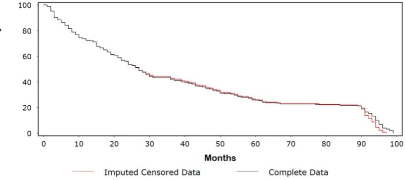
values occurring early in the study. Figure 1 shows a Kaplan-Meir (KM) plot comparing the original
76
censored data with the dataset of complete follow-up times. The probability of surviving 5 years (60
77
months) was ~26% for the original censored data compared with ~18% for the complete dataset. In
78
Figure 2, we compare the complete dataset with the imputed censored dataset. At 5 years, rounding
79
to the nearest whole number, we see that the survival times are identical (i.e., 26%). Indeed, the
80
survival curves are similar until ~90 months, at which point the survival times for the imputed
81
censored time curve are divergently lower than those for the complete dataset. This lack of fit at the
82
extreme end of the KM curves is evident when examining the panel of diagnostic plots in Figure 3.
83
84
85
86
87
Figure 1. Kaplan-Meir (KM) plot comparing the original censored data with the dataset
of complete follow-up times.
4
88
89
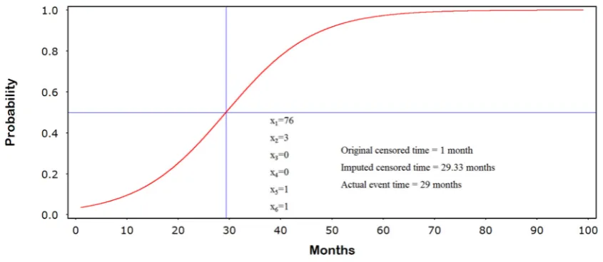
3.2 Generating The Jump-Point Plot
90
The jump-point plot corresponding to covariate pattern
91
= 76, = 3, = 0, = 0, = 1, = 0 (7)
is shown in Figure 4. Here, the variables , ,… , correspond to age (years), grade (I-IV), lymph
92
node invasion (1=yes, 0=no), positive margins (1=yes, 0=no), no hormone therapy (1=yes, 0=no), and
93
no radiation therapy (1=yes, 0=no), respectively. We see that the imputed censored follow-up time of
94
29.33 months closely matches the actual event time of 29 months. This observation was originally
95
censored at 1 month.
96
97
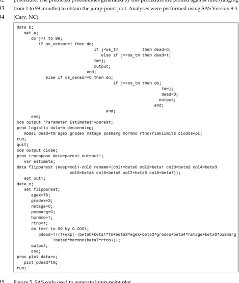
3.3 SAS Code
98
The SAS code use to generate the jump-point plot is shown in Figure 5. In this code, it is assumed
99
that the data contained in Appendix A has been previously read into the dataset “a”. The counting
100
process variables are created in dataset “b” and then modeled using the “PROC LOGISTIC”
101
Figure 3. Diagnostic plots. A: Residual by predicted values; B: RStudent by Jacobian
leverage; C: Expected raw residuals by predicted values.
procedure. The predicted probabilities generated by this procedure are plotted against time (ranging
102
from 1 to 99 months) to obtain the jump-point plot. Analyses were performed using SAS Version 9.4.
103
(Cary, NC).
104
Figure 5. SAS code used to generate jump-point plot.
105
4. Discussion
106
In this manuscript we have introduced a simple method to partially correct for nonignorable
107
early censoring. By rearranging the data as a counting process we are able to account for the
follow-108
up times of all patients, regardless of their censoring status. For example, if a patient is censored at
109
50 months, the counting process creates 50 observations corresponding to each month and
110
accordingly assigns the value of 0 to an indicator variable. On the other hand, if the patient had an
111
event at 50 months, the counting process would create 49 observations with the indicator variable set
6
to 0 and similarly create new observations for each month thereafter until the last month of the study,
113
but instead assigning the value of 1 to the indicator variable.
114
These counting responses are then analyzed with logistic regression, or another appropriate
115
model for fitting binary data. In addition to including outcome related covariates, a variable denoting
116
the time (e.g., month) associated with the indicator variable is added to the model. The predicted
117
value generated by the model for a particular covariate pattern (associated with a censored
118
observation) is then plotted against the time variable (spanning each month of the study) to obtain a
119
jump-point plot. Dropping a line from the midpoint of this plot to the x-axis gives an imputed
120
censored follow-up time. We then replace the original censored time with this value if it larger of the
121
two values. Also, the imputed value is constrained by a natural upper bound to prevent impossible
122
censored follow-up times (e.g., the value must be consistent with a patient’s maximum biologic
123
lifespan).
124
An important aspect of this technique is identifying a well-fitting model for the counting process
125
data so that it is able to accurately predict if the outcome is 0 or 1. Understanding the dynamics of the
126
disease or process under study will aid in the selection of appropriate outcome-related covariates.
127
However, formally testing for model goodness of fit is not practical given the highly correlated nature
128
of the counting process data. In theory, while it may be possible to assess model goodness of fit for
129
dependent data using a robust “Huber-White” approach, the regularity conditions for such estimates
130
are quite stringent [16-18]. Instead, we recommend using leverage and residual diagnostic plots to
131
rule out ill-fitting models [11-13]. In some cases, including power and trigonometric terms into the
132
model may potentially improve the efficiency of the fitting algorithm.
133
The advantage of using a counting process approach is that the imputed censored follow-up
134
times, when appropriately constructed, will better reflect the survival prospects of those who
135
continued in the study. However, because the method is modeled based, it may not be suitable for
136
small datasets or those lacking a set of reasonably predictive covariates. Additionally, it may not
137
always be possible to identify a well-fitting model if there are abrupt changes in the hazard function
138
of the underlying data. The method at hand should not be used if patients who enroll later in study
139
survive longer (e.g., treatment improves over time) or if enrollment criteria change over the course
140
of the study (e.g., worst patients are excluded midway through recruitment) [5].
141
5. Conclusions
142
Overall, the best means for handling informative censoring is to avoid the problem in the first
143
place. Careful planning at the study design stage, routine patient monitoring, and implementing
144
proactive strategies to minimize patient dropout are some important steps to ensure the fidelity of a
145
survival time study.
146
While it was beyond the scope of the current manuscript, it will be informative in future analyses
147
to compare our method with other approaches for dealing with censored values, especially
148
highlighting best and worst-case scenarios [3, 19-24].
149
Acknowledgments: Authors would like to thank the Centre for Clinical Epidemiology and Biostatistics,
150
University of Newcastle, for support and technical assistance during the preparation of this manuscript.
Author Contributions: Jimmy T. Efird and Charulata Jindal conceive and design the project, analyze the data,
152
and wrote the manuscript. Both authors approved the final version of the manuscript.
153
Conflicts of Interest: The authors declared no conflict of interest.
154
155
8 Appendix A. Example cancer dataset (N=250)
Appendix A (Continued)
158
159
160
161
162
163
164
165
166
167
168
169
170
171
172
A=Observation number, B=Age, C=Grade, D= Lymph node invasion, E=Positive margin, F=No
173
hormonal therapy, G=No radiation therapy, H=Actual follow-up time, I=Original censored time,
174
J=Imputed censored time, K=Censoring variable.
175
176
References
177
1. Ranganathan, P.; Pramesh, C. S., Censoring in survival analysis: Potential for bias. Perspect Clin Res 2012, 3
178
(1), 40.
179
2. Lagakos, S. W., General right censoring and its impact on the analysis of survival data. Biometrics 1979, 35
180
(1), 139-56.
181
3. Wu, M. C.; Carroll, R. J., Estimation and Comparison of Changes in the Presence of Informative Right
182
Censoring byModeling the Censoring Process. Biometrics 1988, 44 (1), 175-188.
183
4. Leung, K. M.; Elashoff, R. M.; Afifi, A. A., Censoring issues in survival analysis. Annu Rev Public Health
184
1997, 18, 83-104.
185
5. Zhang, J.; Heitjan, D. F., Nonignorable censoring in randomized clinical trials. Clin Trials 2005, 2 (6), 488-96.
186
6. Shih, W., Problems in dealing with missing data and informative censoring in clinical trials. Curr Control
187
Trials Cardiovasc Med 2002, 3 (1), 4.
188
7. Miettinen, O. S., Survival analysis: up from Kaplan-Meier-Greenwood. Eur J Epidemiol 2008, 23 (9), 585-92.
189
8. Collett, D., Modelling Survival Data in Medical Research. Third ed.; Taylor & Francis group: Florida, USA,
190
2015.
10
9. Blizzard, L.; Hosmer, D. W., Parameter estimation and goodness-of-fit in log binomial regression. Biom J
192
2006, 48 (1), 5-22.
193
10. Hilbe, J. M., Negative Binomial Regression. Second ed.; Cambridge University Press: 2011.
194
11. Laurent, R. T. S.; Cook, R. D., Leverages and Superleverages in Nonlinear Regression. J Am Stat Assoc 1992,
195
87 (40), 985-990.
196
12. Laurent, R. T. S.; Cook, R. D., Leverages, Local Influence, and Curvature in Nonlinear Regression. Biometrika
197
1993, 80 (1), 99-106.
198
13. Pregibon, D., logistic regression diagnostic Ann. Stat. 1981, 9 (4), 705-724.
199
14. Williams, D., Probability with Martingales. Cambridge University Press: New York, 1991.
200
15. Crowder, M. J.; Kimber, A. C.; Smith, R. L.; Sweeting, T. J., Statistical Analysis of Reliability Data. CHAPMAN
201
& HALL: London, 1991.
202
16. Huber, P. J. (1967). “The Behavior of Maximum Likelihood Estimates under Nonstandard Conditions,”
203
Proceedings of the Fifth Berkeley Symposium on Mathematical Statistics and Probability, vol. I, pp. 221–33,
204
1967.
205
17. White, H., Maximum likelihood estimation of misspecified models. Econometrica 1982, 50 (1), 1-25.
206
18. Freedman, D. A., On The So-Called “Huber Sandwich Estimator” and “Robust Standard Errors”.
207
https://www.stat.berkeley.edu/~census/mlesan.pdf. 2006.
208
19. Diggle, P.; Kenward, M. G., Informative drop-out in longitudinal data analysis. J R Stat Soc Ser C Appl Stat
209
1994, 43 (1), 49-93.
210
20. Plante, J. F., About an adaptively weighted Kaplan-Meier estimate. Lifetime Data Anal 2009, 15 (3), 295-315.
211
21. Hogan, J. W.; Laird, N. M., Model-based approaches to analysing incomplete longitudinal and failure time
212
data. Stat Med 1997, 16 (1-3), 259-72.
213
22. Wu, M. C.; Albert, P. S.; Wu, B. U., Adjusting for drop-out in clinical trials with repeated measures: design
214
and analysis issues. Stat Med 2001, 20 (1), 93-108.
215
23. Wei, L.; Shih, W. J., Partial imputation approach to analysis of repeated measurements with dependent
drop-216
outs. Stat Med 2001, 20 (8), 1197-214.
217
24. Little, R. J. A., Modeling the Drop-Out Mechanism in Repeated-Measures Studies. J Am Stat Assoc. 1995, 90
218
(431), 1112-1121.