www.nonlin-processes-geophys.net/18/941/2011/ doi:10.5194/npg-18-941-2011
© Author(s) 2011. CC Attribution 3.0 License.
Nonlinear Processes
in Geophysics
Multiscale characterization of pore spaces using multifractals
analysis of scanning electronic microscopy images of carbonates
M. S. Jouini, S. Vega, and E. A. Mokhtar
The Petroleum Institute of Abu Dhabi, Abu Dhabi, United Arab Emirates
Received: 18 July 2011 – Revised: 2 November 2011 – Accepted: 3 November 2011 – Published: 14 December 2011
Abstract. Pore spaces heterogeneity in carbonates rocks has
long been identified as an important factor impacting reser-voir productivity. In this paper, we study the heterogeneity of carbonate rocks pore spaces based on the image analysis of scanning electron microscopy (SEM) data acquired at var-ious magnifications. Sixty images of twelve carbonate sam-ples from a reservoir in the Middle East were analyzed. First, pore spaces were extracted from SEM images using a seg-mentation technique based on watershed algorithm. Pores geometries revealed a multifractal behavior at various mag-nifications from 800x to 12 000x. In addition, the singularity spectrum provided quantitative values that describe the de-gree of heterogeneity in the carbonates samples. Moreover, for the majority of the analyzed samples, we found low vari-ations (around 5 %) in the multifractal dimensions for mag-nifications between 1700x and 12 000x. Finally, these results demonstrate that multifractal analysis could be an appropri-ate tool for characterizing quantitatively the heterogeneity of carbonate pore spaces geometries. However, our findings show that magnification has an impact on multifractal dimen-sions, revealing the limit of applicability of multifractal de-scriptions for these natural structures.
1 Introduction
Studying carbonate reservoirs is crucial for the oil industry as they contain around half of the hydrocarbon reserves in the world (Moore, 2001). Unlike sandstones which have mainly homogeneous intergranular pores, the diagenesis of carbon-ate rocks combined with other geological processes crecarbon-ate heterogeneous and complex pore spaces with sizes ranging from micro-meter to centimeters (Zhang et al., 2004). In
Correspondence to: M. S. Jouini
addition, these heterogeneities can be observed over sev-eral scales ranging from micro-meter to hundred of meters. Moreover, the geometry and the heterogeneity of carbonate pores can greatly impact the rock physics properties. For example, recent experiments reveal that pore spaces hetero-geneity can cause variations in elastic properties values with as much as 40 % change for the same total volume of pores (Xu and Payne, 2009). Furthermore, pore spaces geometries and heterogeneities can highly impact the transport proper-ties (Payne et al., 2010; Weger et al., 2009). These obser-vations indicate that the relationship between pore spaces structure and rock properties can be highly complex, which makes their modeling a challenging issue. Nowadays, im-age acquisition and analysis techniques represent powerful nondestructive tools that make it possible to quantify the to-tal porosity volume, morphologies and size distribution of pore spaces in porous media. This digital description can be used as input for mathematical models analysing pore distributions from images in order to provide some quan-titative descriptors for heterogeneity. This characterization needs a good specimen preparation and acquisition technique to produce representative images. Scanning electron mi-croscopy (SEM) has been widely used as imaging acquisi-tion technique providing high resoluacquisi-tion images of rock sam-ples and suitable distinction between solid particles and pores (Bogner et al., 2007; Joos et al., 2011; Nadeau and Hurst, 1991). These images consist on grey level pixels, where pore spaces are represented by low levels whereas grains are rep-resented by high level ones. In addition, the measurement of geometrical parameters requires a robust and reproducible segmentation algorithm in order to separate the void phase (pore spaces) from the solid phase (grains).
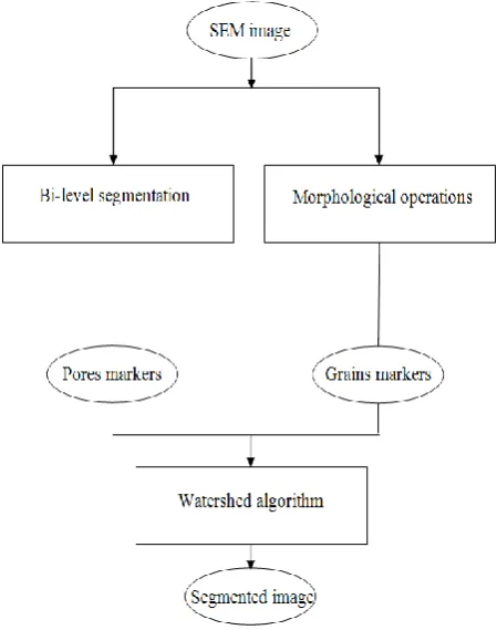
The aim of this paper is to study pore spaces distribu-tion in SEM images of carbonates rocks using a multi-scale characterization. To accomplish this, we first provide an image analysis procedure to automatically detect pore spaces (Fig. 1). Then we use the concept of fractality as a
Fig. 1. Proposed workflow for pore spaces analysis: (a) Acquired SEM image, (b) Segmentation process based on a combination of statistical and spatial approaches, (c) Pore shapes analysis using multifractals and geometrical distributions of areas and aspect ratio.
21 1
Figure 2. Image segmentation workflow based on statistical and spatial method. 2
3
Fig. 2. Image segmentation workflow based on statistical and spatial method.
quantitative description method of the heterogeneity of pore spaces geometry. Finally, as SEM images were acquired at several magnifications, we analyse carbonate pores spaces at different scales to assess the magnification impact on the sample porosity and the heterogeneity descriptors.
In order to solve the segmentation problem of grey level images, authors have used either statistical or spatial methods (Electron, 2004; Ramlau and Ring, 2007). The histogram-based technique (Sahoo et al., 1988; Glasbey, 1993) is one of the most frequently used approaches in statistical
meth-ods and proposes the finding of suitable thresholds in or-der to segment grey level images, depending on histogram shapes. A simple way to obtain a binary image is to choose a suitable threshold for the grey level distribution. Heilbron-ner and Keulen (2006) adjusted the threshold using a sub-jective criterion based on a visual comparison between the input SEM image of rock sample and the segmented image result. Recently, Joos et al. (2011) proposed the use of a sin-gle value threshold computed automatically using the Otsu’s algorithm (Otsu, 1979) in order to segment SEM images where histogram clearly showed a bi-modal behavior related to pore spaces phase and the solid one. Vogel (1996) sug-gested a more sophisticated segmentation technique based on bi-level thresholding to segment SEM images of soil where there was a partial merge between the pore spaces and grains modes in the histogram. Tsai (1995) proposed computing the maximum curvature to detect the suitable threshold in order to solve the highly complex segmentation problem of uni-modal distributed histograms in a porous media. Other au-thors used spatial methods based on the analysis of local ge-ometrical information in order to segment grey level images. Videla et al. (2007), Malcolm et al. (2007), and Jorgensen et al. (2010) proposed the use of a spatial method based on the watershed technique in order to segment micro tomography grey level images.
Since there is no general solution to segment grey level images, a suitable answer to this problem is to combine sta-tistical and spatial image segmentation techniques to take ad-vantage of both methods (Schulter et al., 2010). The pro-posed methodology in this paper is based on a combina-tion of statistical and spatial methods using mainly water-shed algorithm, bi-level segmentation, morphological opera-tions and region growing techniques (Pratt, 2007; Dougherty, 1992; Henk, 1998; Soille, 1999). The main output is a bi-nary image (black and white) where pixels are classified as pore spaces or grains. It is then possible to compute some statistics related to the distribution of pore spaces surfaces and their aspect ratio. In addition, pore spaces of carbonates rock in general have complex shapes. Thus, heterogeneity
quantification can be an interesting characteristic to compute over the several magnifications SEM acquisitions.
Recently, the fractal approach was introduced to charac-terize complex and heterogeneous geometries. This tech-nique is a powerful tool, proposed by Mandelbrot (1983), to describe quantitatively properties of complex morphologies. Fractal analysis is widely recognized to describe and analyze the scale variability of geometrical distributions over a wide range of scales by computing a single exponent called frac-tal dimension (Schertzer and Lovejoy, 1994). The technique is independent of the image source and the real scale of the features. Moreover, it has been used in many applications of sciences for describing complexity and self-similarity in nature as proposed by Evertsz and Mandelbrot (1992). Mul-tifractal is generalization of a fractal approach applied when a single fractal dimension is not able to describe system ge-ometry and instead computes a whole spectrum of exponents (called singularity spectrum). Several studies of fractals and multifractals related to the analysis of pore spaces distribu-tions in porous media and sedimentary rocks can be found in earth sciences (Block et al., 1991; Grout et al., 1998; Wong and Howard, 1986; Flavio et al., 1998; Krohn, 1988; Hansen, 1988; Pi˜nuela et al., 2007; Tarquis et al., 2003, 2006). Muller and McCauley (1992) compared multifractal spectrum of segmented SEM images with a shape factor related to pores, allowing them to distinguish soil groups associated to differ-ent soil structures. Muller (1996) demonstrated that multi-fractal analysis can be useful to characterize different geo-logical chalk environments. In particular, he observed that the multifractal spectrum of pore space is correlated with air permeability values measured from the corresponding core samples. Dathe and Thullner (2005) analyzed pore spaces in porous media using, respectively, monofractals and multi-fractal approaches where the authors tried to establish a rela-tionship between fractal dimensions of pore spaces and solid phase. In this study, we use the multifractality concept on SEM images of carbonate rocks in order to achieve two main goals: the first is to evaluate pore spaces heterogeneities; the second is to assess the effect of magnification on multifrac-tals descriptors and the estimated porosities.
2 Image processing and segmentation
In this study, we used 60 SEM images from 12 samples of a carbonate reservoir in the Middle East taken at several depths and locations. Five (5) SEM images of each sample were ac-quired at different magnifications by focusing at each step on either the central part or a random location of the sam-ple. The size of images was 1024×1024 pixels; magnifica-tions used for acquisimagnifica-tions ranged between 800x and 12 000x. Pore spaces were detected using the segmentation workflow (explained presently) and porosities were estimated at every magnification scale. We developed the image segmentation algorithm and the multifractal analysis codes using Matlab scripts.
22 1
Figure 3. One dimensional illustration of watershed segmentation principle: a) Grey levels of 2
original image, b) Gradient of the signal with localization of sources (local minima in red), c) 3
Flooding of grey levels from sources and creation of dam when two floods meet (in black), 4
d) Result of the segmentation process: in this example four different regions were detected. 5
6 7
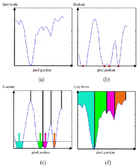
Fig. 3. One dimensional illustration of watershed segmentation principle: (a) Grey levels of original image, (b) Gradient of the sig-nal with localization of sources (local minima in red), (c) Flooding of grey levels from sources and creation of dam when two floods meet (in black), (d) Result of the segmentation process: in this ex-ample four different regions were detected.
In order to segment grey level of SEM images, we used an image processing technique based on applying the water-shed algorithm as a main procedure combined at different steps with statistical and other spatial methods as described by the whole workflow in Fig. 2. Watershed transformation has been widely used in image segmentation problems (Ram-babu and Chakrabarti, 2007; Bieniek and Moga, 2000; Vin-cent and Soille, 1991). In this method, a grey-level image may be considered as a topographic relief where pixel value represents a height. Intuitively, watershed of a relief corre-sponds to the limits of the adjacent catchment basins of water drops. The main idea of this technique is to find local min-imums which will be sources of a continuous water rising flood. Then in order to prevent merging water coming from different sources, a barrier is built at each point of contact. The process ends when the maximum grey level is reached and the union of all those barriers composes the watersheds (Fig. 3). Unfortunately, this transformation creates an over segmentation of the image in most cases. In order to pre-vent this problem, we used an efficient strategy based on us-ing controlled markers (Meyer and Beucher, 1990). These markers aim to help the segmentation process by detecting some zones in pore spaces and in grains which will represent
sources in addition to local minima of the gradient of the image used in the watershed algorithm itself. Markers cor-responding to pore spaces were detected using a bi-level segmentation and a region growing technique. Markers re-lated to grains were obtained using morphological operations (Fig. 4). The bi-level segmentation technique combined with a region growing is a useful segmentation tool for grey level data with histogram partial merge between two main phases. This technique aims in a first step to find two threshold lev-els Gminand Gmax. Hence, in our images segmentation of all
grey levels below the lowest threshold Gminwere detected as
pores and all grey levels above Gmaxwere detected as grains.
These thresholds were computed using gradient masks. So-bel and the Laplace filters were used to compute histograms of grey levels corresponding to detected edges and deduce from them these two thresholds. The second step consisted of using a growing region algorithm to segment the fuzzy in-terval zone (grey levels between Gminand Gmax) using
con-nectivity between pixels belonging to pore spaces. Further-more, morphological operations were applied on the 60 SEM images (from 12 carbonate samples) in order to detect grains markers used as sources for the watershed algorithm. The detected markers represent connected blobs of pixels inside each of the grains zone (Fig. 4c). A series of erosion, opening by reconstruction and closing by reconstruction were used to create flat maxima inside each object. Finally, pixels connec-tivity was used to extract these markers. The final segmen-tation result of the workflow is a binary image where black and white pixels denote respectively grains and pore spaces (Fig. 4e). This result depends on the quality of the detected markers of pore spaces and grains. The next step was to give labels to pore spaces by using connectivity algorithms which allows extracting and evaluating surfaces and aspect ratio of every pore space. Consequently, the final result of this im-ages processing is given by the total pore space, porosity and the pore aspect ratio distribution.
3 Multifractal model
As part of our images analysis, we also studied pore spaces morphologies and heterogeneities based on multifractals. Unlike mathematical definition of ideal fractals, pore spaces structures reveal fractal properties only in a statistical sense, which means we need a statistically representative number of samples to be analyzed. In order to compute a fractal dimen-sion, it is necessary to define a measure in the digital images which is closely associated with pore spaces geometries in images. A widely used measure to study spatial structures is based on the box-counting method (Posadas et al., 2001). The principle is to cover the binary image by a regular square grid partitioning the space into boxes of sizeε. This process is repeated for different box sizes, which is equivalent to an-alyzing the studied geometry or structure at different scales. The main equation for fractal theory establishes a
relation-23 1
2
Figure 4. Watershed segmentation with markers for pores and grains: a) Grey levels input 3
image, b) 3D visualization of image in relief, c) Grains detected markers in red, d) Pores 4
detected markers in blue, e) Final segmentation result: black pixels denote grains and white 5
denote pores. 6
Fig. 4. Watershed segmentation with markers for pores and grains: (a) Grey levels input image, (b) 3-D visualization of image in relief, (c) Grains detected markers in red, (d) Pores detected markers in blue, (e) Final segmentation result: black pixels denote grains and white denote pores.
24 1
2
3
4
5
6
7
8
9
10
Figure 5. Image segmentation of sample S1: a) Original SEM image, b) Binary image result 11
(white pixels for pores and black for grains). 12
13
14
15
16
17
18
(a) (b)
Fig. 5. Image segmentation of sample S1: (a) Original SEM image, (b) Binary image result (white pixels for pores and black for grains).
ship between the number of boxes N(ε)needed to cover the analyzed structure and their sizeε:
N (ε)≈ε−D0 (1)
whereD0is the fractal dimension:
D0=lim
ε→0
log(N (ε))
log(1ε) (2)
The generalization of fractal approach is the multifractal analysis, and is applied when a single fractal dimension is not able to describe system geometry. These objects can be more completely characterized by a spectrum of fractal dimensions. Multifractals are measured using a probability distributionPiin each ith box as:
Pi=εαi (3)
whereε is the box size andαi is the Lipschitz–H¨older ex-ponent characterizing the singularity strength in theith box. The factor αi allows quantifying the distribution complex-ity in spatial location (Posadas et al., 2005). The num-ber of boxes N(α), where the probabilityPi has singularity strengths betweenαandα+dα, can be related to the box size εas:
N (α)=ε−f (α) (4)
where f(α)is the singularity spectrum of boxes characterized with singularityα. For mono-fractal pore distributions,α re-mains constant and the multifractal spectrum is composed of a single point. For multifractal pore distributions, the spec-trum can be represented by a curve with a wide range of val-ues forα. This interval increases with the increase of the
distribution heterogeneity (Posadas et al., 2005; Xie et al., 2010).
Multifractals generalized dimensionsDqof theq−thorder (Hentschel and Procaccia, 1983) are defined as:
Dq=lim ε→0
1
q−1
log(µ(q,ε)) log(ε)
(5) whereµ(q,ε)is the partition function (Chhabra and Jensen, 1989):
µ(q,ε)= N (ε)
X
i=1
Piq(ε) (6)
Moreover, this partition function scales with box sizeεas:
µ(q,ε)=ετ (q) (7)
whereτ(q) is theqthmass exponent and f(α)the singularity spectrum (Halsey et al., 1986), are related as:
τ (q)=(1−q)Dq (8)
f (α)=qα(q)−τ (q) (9)
25 1
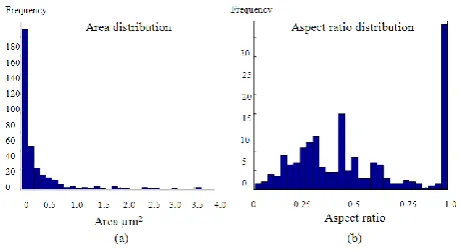
Figure 6. Pore spaces statistics for sample S1: a) Pore spaces size distribution, b) Aspect ratio 2
distribution. 3
4 5 6 7 8 9 10 11 12 13 14 15 16 17 18
Fig. 6. Pore spaces statistics for sample S1: (a) Pore spaces size
distribution, (b) Aspect ratio distribution.
D0,D1andD2can be computed using the following
equa-tions (Posadas et al., 2005):
D0=lim
ε→0
log(N (ε)) log(1ε) , D1
=lim ε→0
N (ε)
P
i=1
µi(ε)log(µi(ε)) log(ε)
,
D2=lim
ε→0
log(C(ε))
log(ε)
(10) whereC(ε)represents the correlation sum.
A first analogy with physical properties appears as D1
and corresponds to the information dimension (Shannon and Weaver, 1949).D0is called capacity dimension and provides
an average related to the information of the analyzed struc-ture distribution (Voss, 1988). D2is the correlation
dimen-sion. Equality for these three dimensions occurs only when the distribution is ideally monofractal (Korvin, 1992).
4 Multifractal analysis of SEM images
4.1 Image analysis
Porosity was computed as a percentage of the segmented pore area to the total image size for the analyzed samples. The segmentation process provides a binary image where black pixels denote the detected grains and the white pixels denote pore spaces. In addition, as no ground-truth informa-tion was available, the resulted detected pores were analyzed visually in order to validate the accuracy of the segmentation process. Figure 5 provides an example of one of the SEM images (sample S1) and the associated segmentation result.
The analyzed zone is a square of 45 µm×45 µm, composed mainly of calcite and revealing a homogeneous distribution of grains and pores. Detected pore spaces in images are in agreement with the expected result based on visual observa-tion. Moreover, these pores are regular and homogeneous and are mainly micro-pores and meso-pores, with a majority
Table 1. Estimation of capacity dimensionD0,information dimensionD1and correlation dimensionD2for samples S1to S12. R2is the
coefficient of determination computed for the linear interpolation in the loglog plot.
Sample Porosity D0 R2 D1 R2 D2 R2
(%)
S1 7.60 1.548 0.995 1.505 0.999 1.492 0.997
S2 17.46 1.661 0.996 1.647 0.998 1.638 0.997
S3 20.66 1.776 0.992 1. 747 0.997 1.733 0.996
S4 16.55 1.681 0.993 1.650 0.996 1.641 0.991
S5 16.05 1.676 0.999 1.638 0.997 1.632 0.992
S6 16.39 1.704 0.995 1.671 0.995 1.655 0.997
S7 7.22 1.537 0.999 1.498 0.994 1.491 0.993
S8 7.92 1.668 0.992 1.585 0.993 1.564 0.996
S9 10.24 1.595 0.996 1.549 0.993 1.541 0.990
S10 7.48 1.633 0.994 1.562 0.997 1.510 0.996
S11 15.37 1.693 0.999 1.649 0.993 1.641 0.992
S12 22.80 1.723 0.998 1.702 0.993 1.694 0.995
26 -8
-7 -6 -5 -4 -3 -2 -1 0
0 0.5 1 1.5 2 2.5 3
S
1q=0
q=1
log(ε)
log
(µ
(q,
ε))
1
-9 -8 -7 -6 -5 -4 -3 -2 -1 0
0 0.5 1 1.5 2 2.5 3
S
2q=0
q=1
log(ε)
lo
g(
µ
(q
,ε
))
2
3
Figure 7. Log-log plots of partition functions (q,) vs for moment order q=0 and q=1 for 4
Sample S1 and Sample S2 respectively in (a) and (b). 5
6
7
8
9
(a)
(b)
Fig. 7. Log-log plots of partition functionsµ(q,ε)vs.εfor moment order q=0 and q=1 for Sample S1and Sample S2, respectively, in (a) and (b).
27
y = 0.0105x + 1.513 R² = 0.6798
1.5 1.55 1.6 1.65 1.7 1.75 1.8
0 5 10 15 20 25
C
apa
ci
ty
di
m
en
si
on
D
O
Porosity
1
2
Figure 8.Linear direct relationship between the capacity dimensions D0 and porosities for all
3
samples. 4
5
6
7
8
9
10
11
Fig. 8. Linear direct relationship between the capacity dimensions
D0and porosities for all samples.
28
1.35 1.4 1.45 1.5 1.55 1.6 1.65 1.7 1.75 1.8 1.85
-5 -4 -3 -2 -1 0 1 2 3 4 5
S
1Multifractal
dimensions
q
Dq
1
2
Figure 9. Multifractal dimensions Dq associated to the SEM image of sample S1 for moments 3
order q between -5 and 5. 4
5
6
7
8
9
10
11
12
13
14
15
16
17
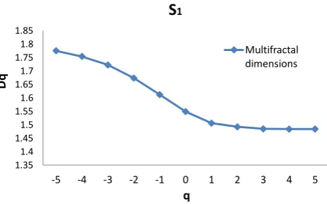
Fig. 9. Multifractal dimensionsDqassociated to the SEM image of sample S1for moments order q between−5 and 5.
29
1
2
3
4
5
6
7
8
9
10
11
12
13
14
15
16
Figure 10. SEM images for samples S
2and S
3(a,c) and respective segmentation results (b, d).
17
White pixels denote pores and black pixel denote grains.
18
19
20
21
22
23
24
25
26
(a) (b)
(c) (d)
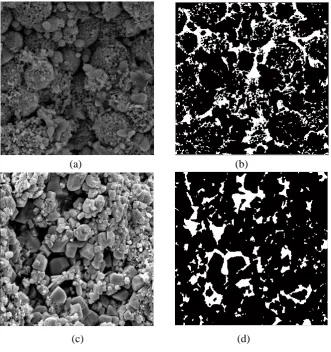
Fig. 10. SEM images for samples S2and S3(a, c) and respective segmentation results (b, d). White pixels denote pores and black pixel
denote grains.
of pore sizes ranging between 0.1 to 1 µm2(Fig. 6a). Further-more, we provide the aspect ratio distribution for the same sample in Fig. 6b. This statistic refers to the ratio between the minor and major axes of an ellipsoidal pore. The aspect ratio distribution for sample S1shows a maximum close to 1.
However, this value is not representative of the whole sample but is generated by the large number of detected micro-pores with sizes close to the image resolution limit.
4.2 Determination of multifractals parameters
The choice of suitable box sizes and range of moments orders are crucial for the multifractal analysis (Saucier and Muller, 1999). In order to find these ranges, we have used two criteria based on assessing the linear behaviors of the mass exponent τ(q) as a function of q and the partition functionµ(q,ε)as a function ofε(Dathe et al., 2006). First, we assessed the variation of the mass exponentτ(q) for several ranges of mo-ments q. We observed thatτ(q) behaves nonlinearly when considering an interval of moments wider than q[−5, +5].
Thus, we chose to restrict our study to this interval where the mass exponentτ(q) versus q is showing a linear relationship with a coefficient of determinationR2above 0.94 (Posadas et al., 2003). Moreover, we found that a moment step equal to 0.5 allows showing accurately the multifractal behavior in the range q[−5, +5]. In addition, we applied the box-counting method to the analyzed images (1024×1024 pix-els) using box sizes ranging from 1 to 1024 and assessed the partition functionµ(q,ε)as function of box sizes. We found a linear behavior relationship with coefficient of determina-tion R2 above 0.9 for box sizes range ε[8, 512] and mo-ments range q[−5, +5]. These ranges were suitable for the majority of analyzed images. Values of multifractal coeffi-cients were determined first by computing slopes of logarith-mic values of the partition function over logarithlogarith-mic values box size as presented in Eq. (5), and second by using the rela-tion presented in Eq. (8). Figure 7 shows the linear behavior of the partition function µ(q,ε)for q = 0 and q = 1 of sam-ples S1and S2. Table 1 provides the capacity dimensionD0,
the information dimensionD1, the correlation dimensionD2,
30 1
2
1.15 1.25 1.35 1.45 1.55 1.65 1.75 1.85
1.3 1.5 1.7 1.9 2.1 2.3
Singularity spectra
S1 S2 S3
α
f(
α
)
3
-15 -10 -5 0 5 10
-5 -4 -3 -2 -1 0 1 2 3 4 5 Mass exponents
S1
S2
S3
q
τ(q
)
4
Figure 11.Plots of the detected pore spaces for samples S1, S2 and S3 (a) and their associated 5
singularityspectra f(α) (b),andmass exponents (c). 6
7
(b) (a)
S1 S2 S3
(c)
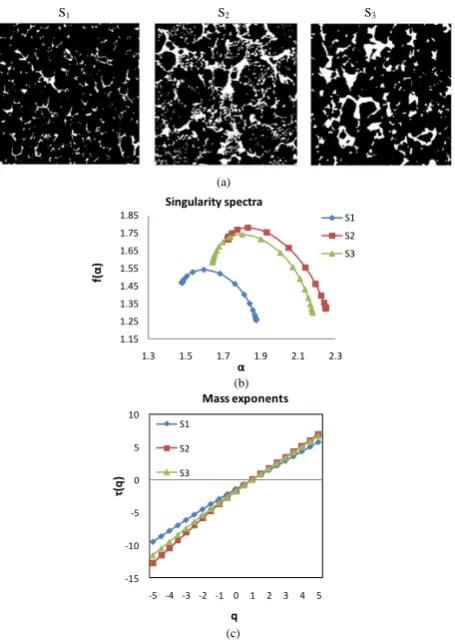
Fig. 11. Plots of the detected pore spaces for samples S1, S2and
S3 (a) and their associated singularity spectra f(α)(b), and mass
exponents (c).
image porosities, and the respective coefficients of determi-nationR2 of the partition function for the twelve analyzed samples for the magnification 12 000x. Furthermore, in or-der to validate the choices made for the moments and the box sizes ranges, we verified that the singularity spectrum f(α) is a concave parabola for each analyzed image show-ing a multifractal behavior. In addition, we also verified that the spectrum touches the internal bisector (f(α)=α)of the axis (Riedi, 1997). The point of intersection between the tan-gent and the graph of f(α) corresponds to f(α(1)) =α(1) =D1
(Evertsz and Mandelbrot, 1992). Moreover, we have investi-gated the possibility of existence of a relationship between the variation of the total porosity and multifractal dimen-sions. Figure 8 reveals a direct linear fitting relationship with a coefficient of determinationR2equal to 0.67 between porosity and the capacity dimensionD0. This observation
suggests that high porosities correspond to high capacity di-mensions. This is an expected result, as for high porosity images the pore spaces structure is more compact, which creases the capacity dimension. In addition, the same in-creasing behavior is observed in Table 1 for the information dimensionD1and the correlation dimensionD2.
Neverthe-less, the generalized dimensionsDqforq≥2 do not show a clear tendency that can be correlated to the total porosity. In relatively homogeneous samples, the generalized dimension Dq showed a slow rate decrease leading to a convergence toward a constant value for moments q≥0, as illustrated in Fig. 9 for sample S1. In this example, generalized
dimen-sionsDq are constant for q≥2. This behavior was also ob-served for homogeneous samples S4, S10and S11. Moreover,
the generalized dimensions Dq for the heterogeneous sam-ples S2, S3, S5, S6, S7, S8, S9and S12 revealed a
continu-ous decrease for 0≤q≤5. These two observations corrobo-rate that generalized dimensionsDqcan provide an indicator of data heterogeneity degree, since their values would con-verge to a constant faster in images where pore distributions were less heterogeneous. Furthermore, Posadas et al. (2005) have shown that homogeneous multifractal distributions have a narrow concave f(α)-spectra, whereas the opposite is true for heterogeneous structures. Thus, the wider is the magni-tude of change of f(α) around the value f(α(0)), the higher is the heterogeneity of analyzed structures. A visual inter-pretation of our segmented images qualitatively reveals more heterogeneity in samples with wider f(α)-spectra, which cor-roborates previous studies. Figures 10 and 11a provides the segmented images of samples S1, S2, and S3. Figure 11b and
c shows respectively their f(α)-spectra and their mass expo-nentsτ(q) with coefficients of determinations, respectively, 0.998, 0.995 and 0.999. For instance, sample S1f(α)-spectra
showed a narrower shape compared to samples S2 and S3,
with a computed interval ofα[1.48, 1.87] and1α=αmax–
αmin= 0.39. Whereas, the singularity spectra revealed higher
magnitudes of alfa changes ofα[1.64, 2.17] and1α=0.53 for sample S2, andα[1.72, 2.24] and1α= 0.51 for sample
S3.
4.3 Scale effect
The magnification at which images are investigated in car-bonate rocks may affect the physical interpretation, in terms of structures and distributions of the visualized pore spaces. Patterns that can be distinguished at a certain image size and magnification may be not present at others. Zhi-bin Liu et al. (2005) studied the magnification effects on the interpreta-tion of SEM images of expansive soils and provided a range of validity for fractal dimensions variations depending on im-age magnification. Therefore, we studied the magnification effect on SEM images in order to evaluate the variations in multifractal dimensions and the total porosity.
4.3.1 Scale effect on multifractal dimensions
Dimensions were computed for the 12 samples at magni-fications ranging from 800x to 12 000x. We found that, for most of analyzed samples, the variation of multifrac-tal dimensions was relatively low, around 5 % in interme-diate magnifications (1700x to 12 000x). Figure 12 shows
1
Figure 12.
Sample S
1acquired at five magnifications: 12000x (M
1), 5600x (M
2), 3000x (M
3),
2
1700x (M
4) and 800x (M
5).
3
4
5
6
7
8
9
10
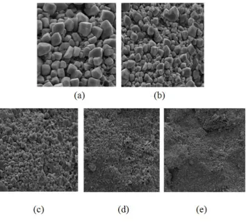
Fig. 12. Sample S1acquired at five magnifications: 12 000x (M1), 5600x (M2), 3000x (M3), 1700x (M4)and 800x (M5).
Table 2. The mean of multifractal dimensions variations, for q≥0, for all samples and the variation of the factorα. The first column shows samples names. The second shows the mean of variations for intermediate magnifications only (magnifications 1700x to 12 000x). The third column provides the mean of variations including the lower magnification (800x). The following columns recapitulate the variation of the factorαfor the five magnifications for each sample. (NM: Non multifractal).
Sample Mean Mean 12 000x 5600x c 3000x 1700x 800x
variation variation 1α 1α 1α 1α 1α
(%) (%)
S1 5.76 13.95 0.402 0.391 0.386 0.428 0.203
S2 1.61 3.58 0.289 0.482 0.522 0.537 0.462
S3 8.00 8.00 NM 0.524 0.524 0.584 0.368
S4 5.21 11.37 0.460 0.420 0.390 0.560 0.442
S5 5.80 5.80 0.458 0.458 0.522 0.396 0.430
S6 2.11 2.95 NM 0.507 0.483 0.494 0.470
S7 1.67 6.02 0.287 0.133 0.333 0.470 0.381
S8 8.31 10.7 NM 0.441 0.405 0.338 0.502
S9 4.81 6.89 0.491 0.359 0.466 0.443 0.432
S10 0.90 3.26 0.523 0.490 0.381 NM NM
S11 1.87 5.92 0.380 0.410 0.430 0.544 0.537
S12 6.07 6.14 0.368 0.265 0.432 0.408 0.383
32
1.3 1.4 1.5 1.6 1.7 1.8
-5 -4 -3 -2 -1 0 1 2 3 4 5
S
1M1 M2 M3 M4 M5
q
Dq
1
Figure 13.Results of multifractal analysis for sample S1. Plots of multifractal dimension Dq
2
versus moment q, qє[-5, 5], at magnifications: 12000x (M1), 5600x (M2), 3000x (M3), 1700x 3
(M4) and 800x (M5). 4
5 6 7 8 9 10 11 12 13 14 15 16
Fig. 13. Results of multifractal analysis for sample S1. Plots of
multifractal dimensionDqversus moment q, q[−5, 5], at magnifi-cations: 12 000x (M1), 5600x (M2), 3000x (M3), 1700x (M4)and
800x (M5).
the sample S1 acquired at five magnifications, and Fig. 13
provides its associated multifractal dimensions. The average variation of multifractal dimensions between magnifications M1(1700x) and M4(12 000x) was equal to 5.76 % for q≥0
for sample S1. Table 2 recapitulates these results for all
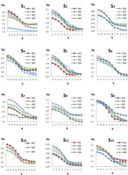
sam-ples and provides the variation of alpha (1α)for all images having multifractal behavior. In Fig. 14, we provide the mul-tifractal dimensions results for all the other analyzed samples at these five magnifications. For the majority of samples, the lowest magnification M5(800x) showed significant variations
in multifractal dimensions between 2.3 % and 13.95 % for the worst case when compared to the other scales. This mag-nification corresponds to the highest scale of visualization and represents the lowest magnification from which detected patterns were most likely related to macro-pores and mega-pores with an equivalent pore radius ranging, respectively, from 2 to 10 µm and from 10 to 100 µm. Furthermore, we found that no clear multifractal behavior could be detected for three samples at the highest magnification S3, S3and S8
as their respective spectra f(α)failed to show a concave shape (Riedi, 1997). The main reason is that the detected patterns at this magnification showed very irregular pores, which are unrepresentative of the general pore spaces distribution ob-served for the other magnifications.
These findings show that magnification has an impact on multifractal dimensions, revealing the limit of applicabil-ity of multifractal descriptions for natural structures, which seem to have multifractal behavior for a limited range of ob-servations scales. Moreover, it corroborates the study of Zhi-bin Liu et al. (2005). In our case, the ratio between magnifi-cations providing significant estimations for multifractal di-mensions was 0.14 (ratio between magnifications 1700x and 12 000x). This result indicates that future studies should be orientated to investigate self similarity for higher scales and its limits.
4.3.2 Scale effect on porosity
We also studied the scale effect on porosity estimation from the segmented SEM images. We found that porosity had an increasing behavior with image magnifications for nine sam-ples and a decreasing behavior for the other three. Figure 15 shows the porosity estimations for samples S1, S2 and S3
for the five magnifications. First, in terms of image analy-sis, the decreasing behavior was expected for samples com-posed mainly of micro-pores and meso-pores, with an equiv-alent pore radius ranging, respectively, from 0.1 to 0.5 µm and from 0.5 to 2 µm, like samples S1and S2. Indeed, for
lower magnifications, micro-pores and meso-pores were less visible and therefore less detectable by the segmentation al-gorithm. Second, the increasing behavior of the other sam-ples was related to the detection of macro-pores and mega-pores. Sample S3, for example, revealed at the lowest
mag-nifications some pores with an equivalent radius larger than 12 µm. Finally, we investigated the possibility of a correla-tion between the variacorrela-tion of multifractal dimensions for the five magnifications and the variation of porosities for these magnifications, but unfortunately we did not find any clear correlation between them.
5 Conclusions
The image analysis techniques presented in this paper allow studying pores morphologies using a grey level image as in-put data without any a priori required for images source. The proposed study showed how useful the multifractal analysis could be when investigating spatial features in highly com-plex geometry images. This paper indicates that the pore space of the analyzed carbonates samples is multifractal and their heterogeneity can be quantified through the variation of the singularity α. In addition, multifractality behavior was detected over a limited range of magnifications (mag-nifications between 1700x and 12 000x). Thus, we could provide a range of scales for the multifractal modeling va-lidity. We also focused on the scale effect on the porosity estimation from the segmented SEM images. We found that porosity showed an increasing behavior with image magnifi-cation, increasing for nine samples and a decreasing for the other four samples. However, no clear correlation could be found between the variations of multifractal coefficients and the variations of porosities due to the magnifications effect. Finally, future acquisitions of thin sections and X-ray com-puted tomography scans for the same samples will be con-ducted in order to study the behavior of detected carbonates pore spaces at higher scales and to compare them to our ac-tual results.
33
1.3 1.4 1.5 1.6 1.7 1.8-5 -4 -3 -2 -1 0 1 2 3 4 5
S
1 M1 M2 M3 M4 q Dq 1.6 1.7 1.8 1.9 2 2.1-5 -4 -3 -2 -1 0 1 2 3 4 5
S
2 M1 M2 M3 M4 q Dq 1.55 1.65 1.75 1.85 1.95 2.05-5 -4 -3 -2 -1 0 1 2 3 4 5
S
3 M2 M3 M4 M5 q Dq1
1.5 1.6 1.7 1.8 1.9 2-5 -4 -3 -2 -1 0 1 2 3 4 5
S
4 M1 M2 M3 M4 q Dq 1.6 1.7 1.8 1.9 2 2.1-5 -4 -3 -2 -1 0 1 2 3 4 5
S
5 M1 M2 M3 M4 q Dq 1.6 1.7 1.8 1.9 2 2.1-5 -4 -3 -2 -1 0 1 2 3 4 5
S
6 M2 M3 M4 M5 q Dq2
1.4 1.5 1.6 1.7 1.8-5 -4 -3 -2 -1 0 1 2 3 4 5
S
7 M1 M2 M3 M4 q Dq 1.5 1.6 1.7 1.8 1.9 2 2.1-5 -4 -3 -2 -1 0 1 2 3 4 5
S
8 M2 M3 M4 M5 q Dq 1.5 1.6 1.7 1.8 1.9-5 -4 -3 -2 -1 0 1 2 3 4 5
S
9 M1 M2 M3 M4 q Dq3
1.5 1.6 1.7 1.8 1.9 2-5 -4 -3 -2 -1 0 1 2 3 4 5
S
10 M1 M2 M3 q Dq 1.65 1.75 1.85 1.95 2.05 2.15-5 -4 -3 -2 -1 0 1 2 3 4 5
S
11 M1 M2 M3 M4 q Dq 1.3 1.4 1.5 1.6 1.7-5 -4 -3 -2 -1 0 1 2 3 4 5
S
12 M1 M2 M3 M4 q Dq4
Figure 14.
Results of multifractal analysis for the 13 samples. Plots of multifractal dimension
5
D
qversus moment q, q
є
[-5, 5], at magnifications: 12000x (M
1), 5600x (M
2), 3000x (M
3),
6
1700x (M
4) and 800x (M
5).
7
8
Fig. 14. Results of multifractal analysis for the 13 samples. Plots of multifractal dimensionDqversus moment q, q[−5, 5], at magnifica-tions: 12 000x (M1), 5600x (M2), 3000x (M3), 1700x (M4) and 800x (M5).
34 y = 0.0001x + 5.997
R² = 0.1174
0 1 2 3 4 5 6 7 8 9
0 2000 4000 6000 8000 10000 12000 14000
P
or
os
ity
(%)
Magnification (x) S1
1
y = 0.0006x + 10.393 R² = 0.6205
0 5 10 15 20
0 2000 4000 6000 8000 10000 12000 14000
P
o
ro
si
ty
(%)
Magnification (x) S2
2
y = -0.001x + 22.613 R² = 0.5724
0 5 10 15 20 25 30
0 2000 4000 6000 8000 10000 12000 14000
P
or
os
ity(
%)
Magnification (x) S3
3
Figure 15.Magnification effect on porosity: Porosity estimation for samples S1, S3 and S3 for 4
magnifications between 800x and 12000x. 5
6
Fig. 15. Magnification effect on porosity: Porosity estimation for samples S1,S3 and S3 for magnifications between 800x and
12 000x.
Acknowledgements. We would like to thank our team in the
Petroleum Institute of Abu Dhabi and more specifically, Melina Miralles for helping to prepare and acquire SEM images for this study. We would like also to thank ADNOC, ADCO, PI, ADMA, ZADCO and the Oil R&D Sub Committee for their support to our research.
Edited by: R. Donner
Reviewed by: S.-A. Ouadfeul and another anonymous referee
References
Bieniek, A. and Moga. A.: An efficient watershed algorithm based on connected components, Original Research Article Pat-tern Recognition, 33, 6, 907–916, 2000.
Block, A., Von Bloh, W., Klenke, T., and Schellnhuber, H. J.: Mul-tifractal analysis of the microdistribution of elements in sedimen-tary structures using images from scanning electron microscopy and energy dispersive X ray spectrometry, J. Geophys. Res., Solid Earth, 96, 223–230, 1991.
Bogner, A., Jouneau, P. H., Thollet, G., Basset, D., and Gauthier, C.: A history of scanning electron microscopy developments: Towards wet-STEM imaging, Microscopy of Nanostructures, 38, 390–401, 2007.
Chhabra, A. B. and Jensen R. V.: Direct determination of the f(α)
singularity spectrum, Phys. Rev. Lett., 62, 1327–1330, 1989. Dathe, A. and Thullner, M.: The relationship between fractal
prop-erties of solid matrix and pore space in porous media, Geoderma, 129, 279–290, 2005.
Dathe, A., Tarquis, A. M., and Perrier, E.: Multifractal analysis of the pore and solid phases in binary two-dimensional images of natural porous structures, Geoderma, Fractal Geometry Applied to Soil and Related Hierarchical Systems – Fractals, Complexity and Heterogeneity, 134, 3–4, 2006.
Dougherty, E. R.: An Introduction to Morphological Image Pro-cessing, SPIE Press, Bellingham, 1992.
Electron, J.: Survey over image thresholding techniques and quanti-tative performance evaluation, J. Electro. Imaging, 13, 146–165, 2004.
Evertsz, C. J. G. and Mandelbrot, B. B.: Multifractal measures, Chaos and Fractals: New frontiers of Science, Springer-Verlag, New York, 921–953, 1992.
Flavio, S. A., Stefan, L., and Gregor, P. E.: Quantitative charac-terization of carbonate pore systems by digital image analysis, AAPG Bulletin, 10, 1815–1836, 1998.
Glasbey, C. A.: An analysis of histogram-based thresholding algo-rithms, Graph Models Image Process, 55, 532–537, 1993. Grout, H., Tarquis, A. M., and Wiesner, M. R.: Multifractal analysis
of particle size distributions in soil, Environ. Sc. Tech., 32, 1176– 1182, 1998.
Halsey, T. C., Jensen, M. H., Kadanoff, L. P., Procaccia, I., and Shraiman, B. I..: Fractal measures and their singularities: The characterization of strange sets, Phys. Rev., 33, 1141–1151, 1986.
Hansen, J. P. and Skjeltorp, A. T.: Fractal pore space and rock per-meability implications, Phys. Rev., 38, 2635–2638, 1988. Henk, J. A. M. and Jos, B. T. M.: Mathematical morphology and
its applications to image and signal processing, Proceedings of the 4th international symposium on mathematical morphology, Kluwer Academic Publishers, 1998.
Heilbronner, R. and Keulen, N.: Grain size and grain shape analysis of fault rocks, Tectonophysics, 427, 199–216, 2006.
Hentschel, H. G. E. and Procaccia, I.: The infinite number of gen-eralized dimensions of fractals and strange attractors, Nonlin. Phen., 8, 435–444, 1983.
Joos, J., Carraro, T., Weber, A., and Ivers-Tiffee, E.: Reconstruc-tion of porous electrodes by FIB/SEM for detailed microstruc-ture modeling, J. Power Sources, 196, 7302–7307, 2011. Jorgensen, P. S., Hansen, K. V., Larsen, R., and Bowen, J. R.: A
framework for automatic segmentation in three dimensions of
microstructural tomography data, Ultramicroscopy, 110, 216– 228, 2010.
Korvin, G.: Fractal models in the earth sciences, Earth-Sci. Rev., Elsevier, 34, 271, 1992.
Krohn, C.: Fractal Measurements of Sandstones, Shales, and Car-bonates, J. Geophys. Res., 93, 3297–3305, 1988.
Liu, Z., Inyang. H., and Cai, Yi.: Magnification effects on the in-terpretation of SEM images of expansive soils, Eng. Geol., 78, 89–94, 2005.
Malcolm, A., and Leong, H., Spowage, A., and Shacklock, A.: Im-age segmentation and analysis for porosity measurement, Journal of Mater. Process. Tech., 6, 192–193, 2007.
Mandelbrot, B. B.: The Fractal Geometry of Nature, Freeman, New York, 1983.
Meyer, F. and Beucher, S.: Morphological segmentation, Journal of Visual Communication and Image Representation, 1, 21–46, 1990.
Moore, C. H.: Carbonate Reservoirs: Porosity Evolution and digen-esis in a sequence stratigraphic framework, Elsevier, Amsterdam, 2001.
Muller, J. and McCauley, J. L.: Implication of fractal geometry for fluid flow properties of sedimentary rocks, Transport in Porous Media, 8, 133–147, 1992.
Muller, J.: Characterization of pore space in chalk by multifractal analysis, J. Hydrol., 187, 215–222, 1996.
Nadeau, P. H. and Hurst, A.: Application of back-scattered electron microscopy to the quantification of clay mineral microporosity in sandstones, J. Sediment. Petrol., 61, 6, 921–925, 199l. Otsu, N.: A threshold selection method from gray-level histograms,
Systems, Man, and Cybernetics Society, 9, 62–66, 1979. Payne, S. S., Wild, P., and Lubbe, R.: An integrated solution to
rock physics modelling in fractured carbonate reservoirs, Society of Exploration Geophysicists, 29, 358, 2010.
Posadas, A. N. D., Gimenez, D., Bittelli, M., Vaz, C. M. P., and Flury, M.: Multifractal characterization of soil particle-size dis-tributions, Soil Sci. Soc. Am. J., 5, 1361–1367, 2001.
Posadas, A. N. D., Gimenez, D., Quiroz, R., and Protz, R.: Multi-fractal characterization of soil pore systems, Soil Sci. Soc. Am. J., 67, 1361–1369, 2003.
Posadas A. N. D., Quiroz R., and Zorogast´ua, P. E.: Multifractal characterization of the spatial distribution of ulexite in a Bolivian salt flat, Int. J. Remote Sens., 26, 615–627, 2005.
Pi˜nuela, J. A., Andina, D., McInnes, K. J., and Tarquis, A. M.: Wavelet analysis in a structured clay soil using 2-D images, Non-lin. Processes Geophys., 14, 425–434, doi:10.5194/npg-14-425-2007, 2007.
Pratt, W. K.: Digital Image Processing 4th Edition, John Wiley & Sons, Inc., Los Altos, California, 2007.
Rambabu, C. and Chakrabarti, I.: An efficient immersion-based wa-tershed transform method and its prototype architecture, J. Syst. Architect., 53, 210–226, 2007.
Ramlau, R. and Ring, W.: A mumford-shah level-set approach for the inversion and segmentation of x-ray tomography data, J. Comput. Phys., 5, 221–539, 2007.
Riedi, R.: Multifractals: an Introduction, Research report, Rice University, 1997.
Shannon, C. E. and Weaver W.: The mathematical theory of com-munication, University of Illinois Press, USA, 1949.
Sahoo, P. K., Soltani, S., Wong, A. K. C., and Chen, Y.: A survey of thresholding techniques, Computer Graph Image Process, 41, 233–260, 1988.
Saucier, A. and Muller, J.: Textural analysis of disordered materials with multifractals, Physica A, 1, 221–238, 1999.
Schertzer, D. and Lovejoy, S.: EGS Richardson AGU Chapman NVAG3 Conference: Nonlinear Variability in Geophysics: scal-ing and multifractal processes, Nonlin. Processes Geophys., 1, 77–79, doi:10.5194/npg-1-77-1994, 1994.
Schulter, S., Weller, U., and Vogel, H. J.: Segmentation of X-ray microtomography images of soil using gradient masks, Comput. Geosci., 36, 1246–1251, 2010.
Soille, P.: Morphological Image Analysis, Principles and Applica-tions, Springer-Verlag New York, Inc, 2, 1999.
Tarquis, A. M., Gim´enez, D., Saa, A., D´ıaz, M. C., and Gasc´o, J. M.: Scaling and multiscaling of soil pore systems determined by image analysis, Scaling Methods in Soil Physics, CRC Press, 434, 2003.
Tarquis, A. M., McInnes, K., Keys, J., Saa, A., Garcia, M. R., and Diaz, M. C.: Multiscaling analysis in a structured clay soil using 2D images, J. Hydrology, 322, 236–246, 2006.
Tsai, D.: A fast thresholding selection procedure for multimodal and unimodal histogram, Pattern Recogn. Lett., 16, 653–666, 1995.
Videla, A., Lin, C. and Miller, J.: 3D characterization of individual multiphase particles in packed particle beds by x-ray microto-mography, Int. J. Miner. Process., 84, 321–326, 2007.
Vincent, L. and Soille, P.: Watersheds in Digital Spaces: An effi-cient algorithm based on immersion simulations, Pattern Anal. Appl., 13, 6, 583–598, 1991.
Vogel, H. J. and Kretzschmar, A.: Topological characterization of pore space in soil sample preparation and digital image-processing, Geoderma, 73, 23–38, 1996.
Weger, R. J., Eberli, G. P., Baechle, G. T., Massaferro, J. L. and Sun, Y. F.: Quantification of pore structure and its effect on sonic velocity and permeability in carbonates, AAPG Bulletin, 93, 1297–1317, 2009.
Wong, P. Z. and Howard, J.: Surface Roughening and the Fractal Nature of Rocks, Phys. Rev. Lett., 57, 637–642, 1986.
Voss, R. F.: Fractals in nature: From characterization to simulation, The Science of Fractal Images, Springer-Verlag New York, USA, 21–69, 1988.
Xie, S., Cheng, Q., Zhang, S., and Huang, K.: Assessing mi-crostructures of pyrrhotites in basalts by multifractal analysis, Nonlin. Processes Geophys., 17, 319–327, doi:10.5194/npg-17-319-2010, 2010.
Xu, S. and Payne, M. A.: Modeling elastic properties in carbonate rocks, The Leading Edge, Rock physics, 28, 66–74, 2009. Zhang, L., Bryant, S., Jennings, J., and Arbogast, T.: Multiscale
flow and transport in highly heterogeneous carbonates, Proceed-ings of the 2004 SPE Annual Technical Conference and Exhibi-tion, Houston, Texas, 26–29 September 2004, SPE 90336, 2004.

![Figure 13. Results of multifractal analysis for sample S1. Plots of multifractal dimension versus moment q, qє[-5, 5], at magnifications: 12000x (M1), 5600x (M2), 3000x (M3) and 800x (MFig](https://thumb-us.123doks.com/thumbv2/123dok_us/38143.1504435/10.595.50.284.65.198/figure-results-multifractal-analysis-sample-multifractal-dimension-magnifications.webp)