www.nat-hazards-earth-syst-sci.net/16/1011/2016/ doi:10.5194/nhess-16-1011-2016
© Author(s) 2016. CC Attribution 3.0 License.
Evaluating flood potential with GRACE in the United States
Tatiana Molodtsova1,*, Sergey Molodtsov1,*, Andrei Kirilenko2, Xiaodong Zhang3, and Jeffrey VanLooy3 1Texas A&M University, College Station, Texas, USA
2University of Florida, Gainesville, Florida, USA
3University of North Dakota, Grand Forks, North Dakota, USA *These authors contributed equally to this work.
Correspondence to: Tatiana Molodtsova ([email protected])
Received: 18 October 2015 – Published in Nat. Hazards Earth Syst. Sci. Discuss.: 19 November 2015 Revised: 6 April 2016 – Accepted: 13 April 2016 – Published: 25 April 2016
Abstract. Reager and Famiglietti (2009) proposed an in-dex, Reager’s Flood Potential Index (RFPI), for early large-scale flood risk monitoring using the Terrestrial Water Stor-age Anomaly (TWSA) product derived from the Gravity Re-covery and Climate Experiment (GRACE). We evaluated the efficacy of the RFPI for flood risk assessment over the con-tinental USA using multi-year flood observation data from 2003 to 2012 by the US Geological Survey and Dartmouth Flood Observatory. In general, we found a good agreement between the RFPI flood risks and the observed floods on re-gional and even local scales. RFPI demonstrated skill in pre-dicting the large-area, long-duration floods, especially during the summer season.
1 Introduction
Among the natural disasters, floods rank the first in terms of the total number of people affected and monetary losses (Center for Research on the Epidemiology of Disasters, 2013). Intensive precipitation events have increased during the final decades of the 20th century (Groisman et al., 2005; Alexander et al., 2006; Trenberth, 2011) and are expected to further intensify in the future (Groisman, 2012). In re-sponse, many countries have developed flood alert systems, such as the European Flood Alert System (Bartholmes et al., 2009) and the US National Weather Service Automated Flood Warning System (Scawthorn, 1999). While most of the systems rely on a dense network of gauging stations, over 95 % of all deaths and a significant portion of the eco-nomic losses caused by floods occur in developing countries where ground flood monitoring and management programs
are still inefficient, and the costs of building control infras-tructure such as dams, weirs, embankments and gauging sta-tions can be prohibitive (Tariq, 2011). These problems were demonstrated well during the 2010 flood disaster in Pak-istan (Larkin, 2010), where the deficiencies in flood monitor-ing and the ensumonitor-ing lack of information led to coordination chaos (Hagen, 2011) and contributed towards an estimated USD 35 billion loss in economic impact.
of GRACE water storage anomaly from 2003 to 2012. Stor-age deficit (SDEF)represents the amount of water which stor-age can accommodate before achievingSMAX. The storage deficit was calculated for each cell for each month:
SDEF(t )=SMAX−(t−1), (1)
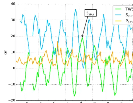
where S(t−1) represents the saturation condition of soil from the previous month. SDEF tells how much additional water a particular area can hold before reaching the maxi-mum capacity and is calculated using the data from the pre-vious month, establishing a potential for forecasting. Exam-ples ofS,SMAXandSDEFestimated for an arbitrary grid cell (52.5◦N, 117.5◦W) are shown in Fig. 1. Normally,SDEF is low/high during the months with high/low precipitation. Fol-lowing Reager and Famiglietti (2009), flood potential (F) for the montht was calculated as
F (t )=PMON(t )−SDEF(t ), (2)
wherePMON(t )is monthly precipitation. The flood potential can be interpreted as the amount of water in excess of the potential water storage. A combination of lowSDEFand high precipitation for the previous month would indicate a high probability of flooding in the current month. Further, RFPI is computed by normalizing the flood potential:
RFPI= F (t )
max[F (t )], (3)
where the maximum of flood potential max[F (t )] is com-puted for each cell of the grid. The values of RFPI vary from−∞to 1, with positive values indicating that water in-put from precipitation is above the mean water storage and should be interpreted as a potential risk for flooding. For val-idation of the RFPI skill we converted the index values to di-chotomous events, where all positive values represent flood potential and all negative values represent absence of the risk. The computed hindcast was validated against the USGS and DFO flood occurrence data, rasterized to a 1◦×1◦ grid of
geographical latitude and longitude.
Monthly data from January 2003 to August 2012 of GRACE RL05 TWSA product (Adam, 2002) from the CSR processing center (http://grace.jpl.nasa.gov) and CPC Merged Analysis of Precipitation (CMAP) (Xie and Arkin, 1997) were used to compute RFPI. Both data sets are gridded at 1◦×1◦. The scaling grid recommended by GRACE Tellus
Figure 1. Variations of total water storage anomaly (TWSA, green
line), monthly precipitation (PMON, blue line) and water storage deficit (SDEF, yellow line) at the grid cell (52.5◦N, 117.5◦W) dur-ing the study period.
data portal (Swenson, 2012) was applied to the GRACE data to account for the attenuation of small-scale surface mass variations (Velicogna and Wahr, 2006).
2.2 Flood observation data
For validation, flood events reported in two observational flood data sets were used: (1) DFO (Brakenridge and Ander-son, 2006) and (2) the US Geological Survey (USGS) Re-trieve Summary of Recent Flood and High Flow Conditions (Hirsch and Costa, 2004). The two data sets differ substan-tially in that the DFO is derived from news and governmen-tal sources and hence mainly refers to large floods in denser-populated regions, whereas the USGS reports are based on in situ stream gauges. In addition, the DFO data started in 1985 but the USGS data are available only since October 2007.
DFO classifies a large flood event in cases of significant damage to structures or agriculture, human life loss and/or long duration. The DFO data were downloaded as a GIS vec-tor data set providing an outline of the area affected by a flood with such attributes as flood dates, duration, fatalities and pri-mary country of flooding. The data were further screened for quality control. For example, in several instances in 2006 and 2009 a mismatch was found between the assigned flood’s ge-ographical coordinates and the primary country of flooding; these events were excluded from our analysis. Finally, vector maps of DFO flood events were rasterized to 1◦×1◦grids. Note that since DFO data are mainly based on media reports, it is expected to bias towards the more densely populated re-gions and/or rere-gions of interest.
USGS station
Cells with less than 5 stations, excluded from the analysis
Figure 2. The distribution of the USGS stream gauging stations (green dots). The blue squares indicate those 1◦×1◦grids containing less than five stations and excluded from the study.
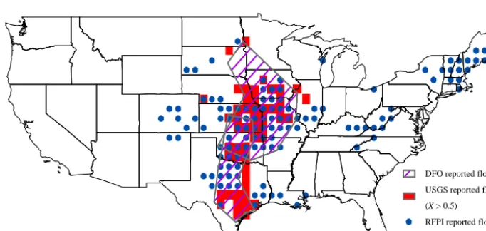
DFO reported flood
USGS reported flood
(X > 0.5) RFPI reported flood
Figure 3. Reported floods in May 2007 by DFO and USGS are compared with RFPI that have positive values.
banks on a daily basis. A flood is further categorized into mi-nor, moderate or major, with number of days in a month in each flood category also reported. Because significant differ-ence exists in spatial scale between GRACE RFPI data and USGS gauge-based flood reports, the USGS data from the individual gauge stations were generalized on a 1◦×1◦grid. First, to ensure statistical significance, all grid cells contain-ing less than five USGS gaugcontain-ing stations were excluded from the analysis (Fig. 2). For those grid cells with more than five stream gauging stations, gauge reports from all the stations within the cell were combined into a monthly flood coeffi-cientX:
X=Dmi+5Dmo+10Dma
N , (4)
whereNrepresents the total number of stations within a cell;
Dmi,DmoandDmaare total numbers of days when the sta-tions within a cell that reported minor, moderate or major floods, respectively. Note that Eq. (4) accounts for flood dura-tion, geographical extent and flood stage. Analyzing several
events from the DFO database and the correspondingX coef-ficient estimated from Eq. (4), we found that areas with cells flagged as flooded withXgreater than 0.5 agreed well with the DFO flood report (Fig. 3). To ensure compatibility be-tween the DFO and USGS generalized flood data, we tested multiple critical values forXand found that usingX=0.5 as an indicator for large flooding minimizes disagreement be-tween the DFO and USGS flooded area observations. Note that the critical valueX=0.5 could mean that 50 % of the gauges reported minor flood for 1 day in a given month, or 10 % of the gauges reported moderate flood for 1 day or 1 % of stations reported major flood for 1 day.
2.3 Forecasting skill assessment
(RFPI) no c(miss, type II error) d(positive rejection) TRP=a/(a+c) FPR=b/(b+d)
for testing the performance of a continuous index (such as RFPI) against binary observational data (e.g., flood or no flood). It uses a binary classifier that maps the index values below and above a certain thresholdτ to the occurrence of an event. Since the exact RFPI threshold value is unknown a priori, the ROC analysis is performed for a range of possible RFPI threshold values. For each threshold, a pair of true pos-itive rate (TPR) and false pospos-itive rate (FPR) was generated by constructing a contingency table (Table 1). A ROC curve plots TPR vs. FPR for different thresholds (Fig. 4) while a 1:1 line represents random guess.
AUC (area under curve) is the area that resides beneath the ROC curve. Since the 1:1 line corresponds to a ran-dom guess, AUC=0.5 relates to no skill and AUC > 0.5 re-lates to better than random skill. Morrison (2005) suggested AUC > 0.7 indicating a strong predictive skill; in practice, the 0.6, 0.7, 0.8 and 0.9 AUC values are frequently used as the thresholds for fair, satisfactory, good and excellent predictive skill. On the ROC plot, the optimal RFPI threshold value τ
corresponds to a location on the ROC curve that is the closest to the (0; 1) point (Fig. 4).
3 Results
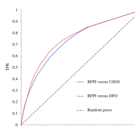
A satisfactory to good agreement was found between the RFPI and the observed floods from both DFO and fil-tered USGS data (i.e., X> 0.5) for the continental USA; AUC=0.75 for the RFPI vs. DFO 2007–2012 flood ob-servations and AUC=0.72 for the RFPI vs. USGS 2003– 2012 flood observations (Fig. 5). The slightly better skill in the RFPI vs. DFO comparison is probably due to the bias in DFO flood observations towards high-damage and large-scale floods. The optimal RFPI threshold values areτ= −0.4 for the USGS andτ= −0.3 for the USGS comparison.
The validation against the USGS data has also demon-strated ability of the RFPI to estimate flood risks at a water-shed level in large flat areas (Fig. 6), e.g., the Great Plains region, with AUC consistently exceeding the 0.7 satisfac-tory predictive skill level. However, we found that over the mountainous and coastal regions the RFPI has a limited abil-ity for flood monitoring (Fig. 6). The resulting ROC curves
0 0.1 0.2 0.3 0.4
0 0.2 0.4 0.6 0.8 1
FPR
Random guess
RFPI perfomance in Tennessee Region
τ=0.3
Figure 4. An example showing the ROC curve estimated for the
Tennessee watershed using different RFPI thresholds. The optimal value of the classifier thresholdτ for this watershed is 0.1, corre-sponding to the point on the ROC curve that is the closest to the (0; 1) point. The dashed line represents random guess, which has an area under the curve (AUC) of 0.5, whereas a predictive index such as RFPI has an AUC > 0.5.
0 0.1 0.2 0.3 0.4 0.5 0.6 0.7 0.8 0.9 1
0 0.2 0.4 0.6 0.8 1
TPR
FPR
FPI versus USGS
FPI versus DFO
Random guess RFPI versus USGS
RFPI versus DFO
Random guess
Figure 5. The ROC curves for RFPI when compared with the
USGS- and DFO-reported floods.
Color Region AUC
Ohio region 0.71
Arkansas – White– Red region 0.72 Lower Mississippi region 0.72
New England region 0.73 Missouri region 0.73
Upper Mississippi region 0.74 South Atlantic Gulf region 0.74 Souris– Red– Rainy region 0.78
Upper Colorado region 0.79 Tennessee region 0.82
Random guess 0.5
0 0.1 0.2 0.3 0.4 0.5 0.6 0.7 0.8 0.9 1
0 0.2 0.4 0.6 0.8 1
T
P
R
FPR
Figure 6. The RFPI predictive skills are evaluated by comparing with USGS-reported floods using ROC curves and AUC values for each of
the major watersheds. The colors of the ROC curve match the colors of the delineated watersheds. The Rio Grande and California watersheds (in white) were excluded due to low number of floods. The watersheds that have RFPI AUC values less than 0.7 are in grey color (Lower Colorado, Texas Gulf, Great Basin, Great Lakes, mid-Atlantic and Pacific Northwest) and not shown in the comparison.
0 0.1 0.2 0.3 0.4 0.5 0.6 0.7 0.8 0.9 1
0 0.2 0.4 0.6 0.8 1
TPR
FPR
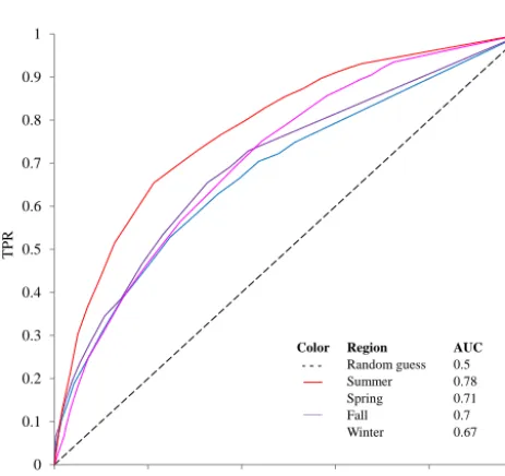
Color Region AUC
Random guess 0.5 Summer 0.78 Spring 0.71
Fall 0.7
Winter 0.67
Figure 7. A seasonal evaluation of RFPI predictive skills (vs. the
USGS-reported floods) for the Mississippi river basin.
Mississippi, Missouri, Ohio, Tennessee and Arkansas-White-Red watersheds; see Fig. 6), AUC is 0.67 in the winter period and 0.78 in the summer.
As a case study, we now examine a wide spread flood that occurred in the northeastern USA due to a series of heavy rain events during March and April 2007 (Fig. 8). Precipita-tion in the region had dropped steadily during the winter of 2006–2007. Surprisingly, the soil moisture deficit (SDEF)had
also decreased during the same period, probably due to melt-ing of the accumulated snow (Fig. 8c). The sudden increase in precipitation in March triggered RFPI (blue squares in Fig. 8a) showing positive values, indicating that the amount of precipitation had exceeded the storage capacity and the region is at risk of potential flooding. The continual increase in precipitation during April caused regional flooding (green polygon in Fig. 8a). The area showing positive RFPI values predicted in March agrees well with the actual flood extent as reported by DFO for the month of April. Also, notice that RFPI estimated in April indicates a much more extended area subject to potential flooding (Fig. 8b). Had the heavy precip-itation continued in May, the flooding would have been much more damaging and would have affected a much wider area than what has been reported by DFO.
4 Discussion
Figure 8. The 2007 flood in the northeastern USA. (a) grid cells with positive RFPI values in March, 1 month before the flooding; (b) grid
cells with positive RFPI values in April, the flooding month; (c) the average storage deficit (blue line) and precipitation (yellow line) over the northeastern USA from October 2006 to September 2007. In (a) and (b), the DFO-reported flood area is shown as green polygon.
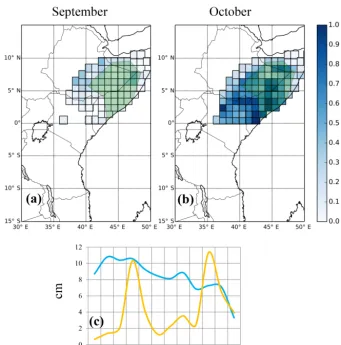
While we have tested the RFPI in the USA where a dense network of flood gauges has been established, potentially greater use of this method is in developing countries, where due to inadequate monitoring capability, floods tend to cause significant damage and the most loss of life. Also, floods in developing countries, as found through the DFO database, are mainly caused by heavy rainfall events, for which the RFPI seems to perform well in predicting flood potential. Therefore, to further evaluate its applicability, we exam-ined the Juba–Shabelle river basin, a 783 000 km2watershed shared between Somalia and Ethiopia. Similar to Fig. 8 we examined a flood caused by a heavy precipitation event over the basin in October 2006, which ranked as the most damag-ing flood in Eastern Africa in 50 years. In Ethiopia, over 150 people died and over 122 500 were displaced; in Somalia, over 80 people died and over 299 000 were displaced (DFO database). We found increasing RFPI in the Juba–Shabelle watershed 1 month prior to the flood (Fig. 9a) and during the month of flood (Fig. 9b), both predictions agreeing well with the actual flood extent area reported by DFO. The time
series of the water storage deficit generated over the water-shed (Fig. 9c) shows a significant decrease of nearly 3 cm in the available water storage capacity in September, 1 month before the damaging flood. Based on this preliminary anal-ysis, we speculate that the developing countries with sparse or inadequate flood monitoring networks are potential bene-ficiaries of this approach.
Figure 9. The 2006 flood in the Juba–Shabelle river basin. (a) Grid cells with positive RFPI values in September, 1 month before the flooding; (b) grid cells with positive RFPI values in October, the flooding month; (c) the average storage deficit (blue line) and precipitation (yellow
line) over the Juba–Shabelle river basin from January 2006 to December 2006. In (a) and (b), the DFO-reported flood area is shown as green polygon.
the Center for Research on the Epidemiology of Disasters (http://www.cred.be/) flood monitoring system.
Data availability
The GRACE Release-5 10/2012 TWSA product was ob-tained from http://grace.jpl.nasa.gov/; the CPC Merged Analysis of Precipitation was obtained from http://disc.sci. gsfc.nasa.gov/giovanni; DFO Global Archive of Large Flood Events data were obtained from http://floodobservatory. colorado.edu/Archives/index.html; the USGS Retrieve Sum-mary of Recent Flood and High Flow Conditions was ob-tained from http://waterwatch.usgs.gov/.
Acknowledgements. The study was supported by NASA grant
NNX10AH20G and UND Summer Graduate Research Professor-ship. X. Zhang acknowledges partial funding support from NSF Grant 1355466. The authors also wish to thank the Editor, Bruno Merz, John T. Reager and an anonymous referee whose suggestions and comments greatly improved the manuscript.
Edited by: B. Merz
Reviewed by: J. T. Reager and one anonymous referee
References
Adam, D.: Gravity measurement: amazing GRACE, Nature, 416, 10–11, 2002.
Alexander, L. V., Zhang, X., Peterson, T. C., Caesar, J., Gleason, B., Tank, K., Haylock, M., Collins, D., Trewin, B., Rahimzadeh, F., Tagipour, A., Kumar, R., Revadekar, J., Griffiths, G., Vin-cent, L., Stephenson, D. B., Burn, J., Aguilar, E., Brunet, M., Taylor, M., New, M., Zhai, P., Rusticucci, M., and Vazquez-Aguirre, J. L.: Global observed changes in daily climate extremes of temperature and precipitation, J. Geophys. Res., 111, D05109, doi:10.1029/2005JD006290, 2006.
drological applications, Transboundary Floods: Reducing Risks Through Flood Management, Nato science series: IV: earth and environmental sciences, 72, p. 1, doi:10.1007/1-4020-4902-1_1, 2006.
Center for Research on the Epidemiology of Disasters: The OFDA/CRED International Disasters Database, available at: www.cred.be (last access: April 2016), 2013.
Chen, J. L., Wilson, C. R., Tapley, B. D., and Ries, J. C.: Low degree gravitational changes from GRACE: vali-dation and interpretation, Geophys. Res. Lett., 31, L22607, doi:doi:10.1029/2004GL021670, 2004.
CPC Merged Analysis of Precipitation: Goddard Earth Sciences (GES) Data and Information Services Center (DISC), NASA, available at: http://giovanni.gsfc.nasa.gov/giovanni/, last access: April 2016.
Fawcett, T.: An introduction to ROC analysis, Pattern Recogn. Lett., 27, 861–874, 2006.
Global Active Archive of Large Flood Events: Dartmouth Flood Observatory, University of Colorado, available at: http:// floodobservatory.colorado.edu/Archives/index.html, last access: April 2016.
GRACE Release-5 10/2012 TWSA product: GRACE Tel-lus, NASA, available at: http://grace.jpl.nasa.gov/data/get-data/ monthly-mass-grids-land/, last access: April 2016.
Groisman, P. Y., Knight, R. W., Easterling, D. R., Karl, T. R., Hegerl, G. C., and Razuvaev, V. N.: Trends in Intense Precipi-tation in the Climate Record, J. Climate, 18, 1326–1350, 2005. Groisman, P. Y.: Changes in intense precipitation over the Central
US, J. Hydrometeorol., 13, 47–66, 2012.
Hagen, E.: Let us create flood hazard maps for developing countries, Nat. Hazards, 58, 841–843, 2011.
Hirsch, R. M. and Costa, J. E.: US stream flow measurement and data dissemination improve, Eos 85, 20, 197–203, 2004.
Murphy, A. and Winkler, R.: A general framework for forecast ver-ification, Mon. Weather Rev., 115, 1330–1338, 1987.
Proud, S. R., Fensholt, R., Rasmussen, L. V., and Sandholt, I.: Rapid response flood detection using the MSG geostationary satellite, Int. J. Appl. Earth. Obs., 13, 536–544, 2011.
Reager, J. T. and Famiglietti, J. S.: Global terrestrial water storage capacity and flood potential using GRACE, Geophys. Res. Lett., 36, L23402, doi:10.1029/2009GL040826, 2009.
Retrieve Summary of Recent Flood and High Flow Conditions: US Geological Survey, available at: http://waterwatch.usgs.gov/?id= wwdp2, last access: April 2016.
Scawthorn, C.: Modeling flood events in the US, Proceedings of the EuroConference on Global Change and Catastrophe Risk Man-agement, International Institute for Advanced Systems Analysis, 6–9 June 1999, Laxenburg, Austria, 1999.
Swenson, S. C.: GRACE monthly land water mass grids NETCDF RELEASE 5.0. Ver. 5.0. PO.DAAC, CA, USA, available at: http: //dx.doi.org/10.5067/TELND-NC005 (last access: April 2016), 2012.
Tariq, M. A. U. R.: Risk-based planning and optimization of flood management measures in developing countries: case Pakistan, doctoral thesis, VSSD, TU Delft, Delft, the Netherlands, 2011. Trenberth, K. E.: Changes in precipitation with climate change,
Clim. Res., 47, 123–138, 2011.
Velicogna, I. and Wahr, J.: Measurements of time-variable gravity show mass loss in Antarctica, Science, 311, 1754–1756, 2006. Xie, P. and Arkin, P. A.: Global precipitation: A 17-year monthly