SHIP MANOEUVRING ASSESSMENT BY USING NUMERICAL SIMULATION APPROACH

(1)

SHIP MANOEUVRING ASSESSMENT

BY USING NUMERICAL SIMULATION

APPROACH

1

C.W. MOHD NOOR*, 1K.B. SAMO, 1W.B. WAN NIK

1

Department of Maritime Technology, Universiti Malaysia Terengganu,

Malaysia.

*Author email: [email protected]

Abstract:

Rapid development in computer technology today has revolutionized the method used to predict ship hydrodynamic complex systems by application of numerical simulation approach. One important prediction technique made feasible by high-speed computers is the time-domain simulation especially in the prediction of ship motions, sea-keeping and also manoeuvring. On the other hand International Maritime Organization (IMO) standard for ship manoeuvrability has hastened the need for more accurate prediction of ship’s manoeuvrability at the early design stage. There are many test methods available for manoeuvring prediction such as free running and captive model tests. However these methods are expensive and time consuming. As an alternative, the numerical simulation method is taking place the current principal approach. This paper presents a manoeuvring assessment of an Offshore Supply Vessel (OSV) based on the numerical time domain simulation approach. Manoeuvring time domain simulation programmed was developed by using Matlab Simulink software. Prediction of vessel swept paths was obtained by double integration of acceleration in the surge, sway and yaw axes. Simulation result shows that the manoeuvring criteria of an OSV comply with the IMO standard.

Keywords: Manoeuvring assessment, Mathematical model, Numerical simulation

1. INTRODUCTION

The development of high-speed computers has revolutionized the method used to predict the behaviour of complex systems and phenomena i.e. time-domain simulation, in which behaviour of a system is determined by numerical integration of a set of equations of motions. Time-domain simulation was widely used in the marine field especially in the prediction of ship motions, sea-keeping and also manoeuvring for all types of ship and marine systems. These simulations used hydrodynamic coefficients based on prediction formulae or test data from captive model test conducted in a towing tank.

Simulation offers several significant advantages over competing technique, such as free running model tests in order to assess vessel controllability and manoeuvring performance. The most important advantages of simulation are that once the initial model test is conducted and simulation model generated, almost any manoeuvre or ship operation can be simulated without additional model tests. The simulation model can be readily and economically modified to determine the effect of changes, such as increasing of rudder and propeller size.

The manoeuvring can be either of the fast-time or real-time type. Fast-time simulation is conducted using autopilot or pre-programmed control. The time required to conduct such simulation depends only on the complexity of the simulation model and the power of the computer. Fast-time simulations could provide a cost effective means for evaluating ship manoeuvrability, controllability and course keeping. Real-time simulations are conducted using a human operator or ship-handler. Some level of simulator, will provide ship state data such as position, heading and velocity. This information made the control of the helm and engine order meaningful for the ship handler. The real-time decision-making provided by the ship - handler is essential for ship handling and waterway design studies.

(2)

an alternative, nowadays the numerical simulation method with parameters determined from a database is taking place the principal approach. The objective of this study was to assess the manoeuvring characteristic of an Offshore Supply Vessel (OSV) by using a numerical approach time domain simulation programme. In general, low speed vessels with high block coefficient such as OSV are known to have bad manoeuvring characteristic because of the full hull form with small length to beam ratio [9].

2. LITERATURE RIVIEW

Final adoption of IMO standards [1] has urged ship designer to establish design criteria in order to satisfy manoeuvrability standards. The IMO standard covers the course-keeping and yaw-checking ability as well as the conventional turning circle and stopping abilities, thus the prediction of course stability has become important. Prediction of the manoeuvring parameters such as advance, transfer, tactical diameter of turning circle and overshoots of zig-zag manoeuvres using simulation program, the mathematical model of manoeuvring motion must be developed together with hydrodynamic derivatives.

More study has been done related to the simulation of the IMO standard ship manoeuvring using mathematical models regression equations based on captive model test results. Inoue [2] considered non-linear coefficients and various load conditions including trim on ship manoeuvring prediction. Kijima [5,6] show that revised Inoue’s formulae which presented new improved regression equation for predicting the hull derivative, the flow straightening factor and wake fraction used in the MMG model based on captive test. The equation is valid for both even keel and trimmed condition.

Lee [9] compared the MMG mathematical manoeuvring model with a typical conventional whole ship model such as the Abkowitz mathematical model. The purpose of introducing a MMG modular simulation model is to split the mathematical model into relevant physical phenomenon, typically a separation of hull forces and rudder propeller-hull interaction forces, but also other mathematical models can be included such as the behaviour of the engine, either a slow or medium speed diesel engine or a turbine. Furthermore, research can be made with individual modules. Kajima [3] presented empirical formulas to calculate all the forces acting on ship hull and the predicted results obtained show good agreement with full scale data.

2.1 IMO Manoeuvring Standards

The problem of ship manoeuvrability has considerably grown in the last decade, both for merchant and naval ships. With regards to merchant ships, the Interim Standards of Ship Manoeuvrability A.751 (18) was adopted as IMO Resolution MSC.137 (76), “Standards for Ship Manoeuvrability” in 76th Marine Safety Committee meeting in December 2002. IMO enforced minimum manoeuvrability criteria to ensure safety of all seagoing ships. These criteria are listed in Table 1 while the manoeuvring indices are shown in Figure 1.

Table 1: IMO evaluation criteria in final standards for ship manoeuvrability [1]

Item Test Criteria

Turning ability Turning test with max. Rudder angle (35o.)

Advance < 4.5L Tactical diameter < 5.0L Initial turning

Ability 10°/10° Z-test

Distance ship run before 2nd rudder execution < 2.5L

Stopping ability Stopping test with

full astern Track reach < 15L

Course-keeping and

yaw-checking ability

10°/10° Z-test

1st overshoot <10° (L/U<10s) <(5+0.5 L/U)o (10s<L/U<30s)

<20° (30s<L/U) 2nd overshoot

<25° (L/U<10s ) <(17.5+0.75(L/U))° (10s<L/U<30s)

<40° (30s<L/U)

(3)

Fig. 1. Turning Ability and Zig-Zag Manoeuvre Indices [10]

3. MATHEMATICAL MODEL

The mathematical model for manoeuvring motion can be structured from the equations of motion with reference to the co-ordinate system, whose origin is the ship’s centre of gravity as shown in Figure 2. (U) is the actual ship velocity that can be resolved into advance velocity (u) and transversal velocity (v). The ship has also a rotation velocity with respect to the Z-axis. This axis is normal to the XY plane and passes through the ship centre of gravity (CG). (β) is the angle between (U) and the X-axis and it is called the drift angle. (Ψ) is

the ship heading angle and (δ) is the rudder angle. In this study, manoeuvrability was approached as a bi-dimensional phenomenon.

Two reference systems used, one of them fixed (Xo, Yo) and the other moving with the ship, with its origin at the centre of gravity. Yaw motion is supposed to occur around this point. In the moving reference, X-axis is positive forward and Y-axis is positive starboard. For both systems, moving and fixed, angles are positive in the clockwise sense.

0

y

0 0

x





Y v,

X u,

 U

N r,

CG

Fig. 2. Co-ordinate System

3.1 Equations of Motion

(4)





















r N

L U r L U U L J I Y r m m U U U L m m X r m m U U U L m m zz zz x y y x                 _                                                                             2 cos cos sin sin sin cos



(1) where:

X’, Y’ : Dimensionless surge and sway force acting on a ship,

N’ : Dimensionless yaw moment acting on a ship,

m’,m’xm’y: Dimensionless mass of ship, and added mass in X and Y-directions,

I’zz : Dimensionless moment of inertia of ship in Z-axis,

J’zz : Dimensionless added moment of inertia of ship in Z-axis, Β : Drift angle at the centre of gravity C.G. [ β = - sin-1(v/U)],

r′ : Dimensionless turning rate [ r = dψ/dt ],

L, T, U : Ship length, draught and speed, respectively.

The superscript {'} in the equations refers to the non-dimensional quantities defined by: L U r r dU L N N LdU Y X Y X d L J I J I J I J I d L m m m m m m xx xx zz zz xx xx zz ZZ y x y x                 2 2 2 4 2 5 . 0 5 . 0 , , 5 . 0 , , , , , , 5 . 0 , , , ,



The left hand-side of equations (1) represents the inertial terms. The right hand-side represents the external forces and moments that act on the ship. These forces and moments can be described separately into the following components:

X’ = X’_H+ X’_R+ X’_P

Y’ =Y’_H+ Y’_R ₍₂₎

N’ = N’_H+ N’_R

The subscripts “H”, “P”, and “R” symbolize ship hull, propeller, and rudder respectively according to the concept of Mathematical Model Group [7,11].

3.2 Forces and Moments Acting on Hull

(5)

hydrodynamic force (X’H), the lateral force (Y’H), and yaw moment (N’H) acting on the ship hull are expressed as follows [3]:

X’H = { X’βr r’ sinβ + X’uu cos2β }

Y’H = { Y’ββ + Y’r r’ + Y’βββ│β│+ Y’rr r’│r’│+ (Y’ββr β + Y’βrrr’) βr’ }

N’H = { N’ββ + N’r r’ + N’βββ│β│+ N’rr r’│r’│+ (N’ββr β + N’βrrr’) βr’ } (3)

3.3 Forces and Moments Induced by Propeller

The hydrodynamic forces generated by the ship propeller are expressed in equation (4), neglecting lateral force and yaw moment that affects the stopping manoeuvre [5,6]:

X’P =[ Ctp ( 1 – tP ) n2 DP4 KT ( JP )]/0.5ρLdU2

Y’P = 0

N’P = 0

 



P

 

P



P

P P P

T

nD w U

J

J C J C C J K

/ 1 cos

2 3 2 1

 

 





(4)

where:

tp : Thrust reduction coefficient in straight forward moving,

Ctp: Propeller constant,

N : Propeller revolution,

Dp : Propeller diameter,

wp : Effective wake fraction coefficient of propeller in straight running,

KT : Thrust coefficient of a propeller force,

Jp : Advance coefficient,

C1, C2, C3: Constants for propeller open characteristics.

3.4 Forces and Moments Induced by Rudder

The hydrodynamic forces generated by ship rudder are described in equation (5), in term of rudder normal force F’N, rudder angle δ and rudder-to-hull interaction coefficient tR, aH and xH :

X’_R = − (1 − tR )F’N sinδ

Y’

R = − (1 + aH )F’N cosδ

N’R = − ( x_R+ aH xH )F’N cosδ (5)

where:

xR : The distance of rudder from the ship centre of gravity,

xH : The distance between the ship centre of gravity and centre of lateral force, δ : Rudder angle,

F’N: Dimensionless rudder normal force,

tR: Rudder deduction fraction,

aH: Interaction coefficient between rudder and a ship hull.

The components of forces in the equation of motion were calculated corresponding to the prescribed manoeuvring motions. The vessel’s swept path can be obtained by simulating the coefficients, which are calculated from the approximate formulae in the equation of motion. The swept path is then obtained by double integrating the acceleration of the vessel in the surge, sway and yaw axis of the mathematical model.

The equations of motion used in the simulation program are described in equation (1). The details of non-dimensional surge force (X’) equation are as follows:







m



r

X

U

L

m

_x _y



























































cos





sin



sin



(6)

Equations (6) were rearranged in order to get the acceleration. Then the equation of accelerations (see equation 7) needs to be double integrating to obtain velocities and finally displacements.









    cos sin sin _U U L m m r m m X U x y                                (7)

The above set of equations (7) could be integrated by using the ode function as follows:









dt

U

L

m

r

m

X

U

x y t t























































_



cos

sin

2 1



(8)









dt

U

L

m

r

m

X

x

x y t t t t























































_



cos

sin

2 1 2 1



(9)

4. SIMULATION PROGRAM

The software used in this study called MATLAB Simulink which the name stands for Matrix Laboratory. MATLAB is a high-performance language for technical computing. It integrates computation, visualization, and programming in an easy-to-use environment and user friendly where problems and solutions are expressed in familiar mathematical notation.

The Simulink feature is a software package for modelling, simulating, and analysing of dynamic systems. It supports linear and non-linear systems, modelled in continuous time, sampled time, or a hybrid of the two. Systems can also be multi-rate, i.e., have different parts that are sampled or updated at different rates. Simulink also provides a Graphical User Interface (GUI) that use various types of elements called blocks to create a simulation of a dynamic system which a system that can be modelled with differential or difference equations whose independent variable is time.

(7)

Fig. 3. Simulation programme flowchart

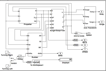
In input block, the programme received input data of rudder angle and hydrodynamic coefficients. These input data will then be used in process block in order to calculate the hull, rudder and propeller forces. The layouts of the process block module are shown in Figure 4.

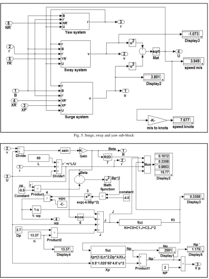
Hull modules are divided into three sub-blocks which are called surge, sway and yaw sub-block. The details are shown in Figure 5. Propeller and rudder forces are calculated in their sub-block as shown in Figures 6 and 7, respectively.

(8)

Fig. 5. Surge, sway and yaw sub-block

(9)

Fig. 7. Rudder sub-block

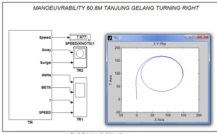
The equation of motion is double integrated to obtain the translation of motion in x and y direction. Lastly the output results of ship path are displayed in graphical form as shown in Figure 8.

Fig. 8. Output result of ship path

5. SIMULATION RESULTS

(10)

Fig. 9. Simulation results of turning circle trajectories to port and starboard

Advance Distance (Ad) and Tactical Diameter (Td) were measured and the summary is tabulated as Table 2. The results showed that both criteria found comply with IMO standards. The purpose of turning manoeuvre is to determine the turning ability and the response of the ship to the deflection of the rudder at 35o angle.

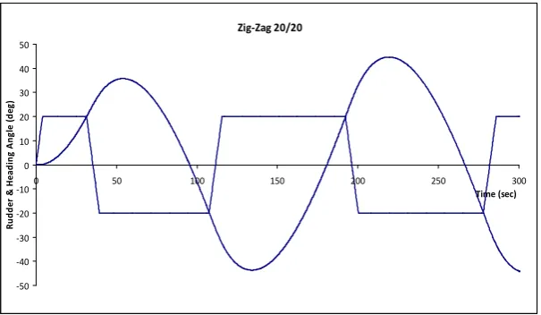
On the other hand, the Zig-Zag manoeuvre was carried out for the purpose of yaw checking ability which represents the inherent effectiveness of the two rudders in making changes of ship heading. The simulation results of Zig-Zag 10/10 and Zig-Zag 20/20 are recorded in Table 3. It shows that the 1st and 2nd overshoot angle of Zig-Zag 10/10 and Zig-Zag 20/20 meets the IMO standard. This means that the OSV had a good yaw checking ability. The details of the simulated time histories for Zig-Zag manoeuvre was plotted in Figures 10 and Figure 11, respectively.

Table 2: Simulation results of turning circle

Parameter Turning (port)

Turning (starboard)

IMO

Criteria Result

Advance distance 3.1 L (188m) 3.2 L (194m) < 4.5 L Comply

Tactical diameter 2.7 L (164m) 2.8 L (169m) < 5.0 L Comply

Table 3: Simulation results of Zig-Zag 10/10 and 20/20

Parameter Zig-Zag 10/10 Zig-Zag 20/20 Result Predict. IMO Predict. IMO

1stovershoot (deg.) 6.5 10 15.7 25 Comply

2nd overshoot (deg.) 10.6 25 23.6 - Comply

Fig. 10. Simulation time histories of Zig-Zag 10/10

Turning Circle ‐ PORT

‐50 0 50 100 150 200 250

‐250 ‐200 ‐150 ‐100 ‐50 0 50

X (m)

Y

(m

)

Turning Circle ‐ STBD

‐50 0 50 100 150 200 250

X (m)

Y

(m

)

Zig‐Zag 10/10

‐25

‐20

‐15

‐10

‐5 0 5 10 15 20 25

0 50 100 150 200 250 300

Time (sec)

Ru

d

e

r

&

He

a

d

in

g

Ang

le

(d

eg

(11)

Fig. 11. Simulation time histories of Zig-Zag 20/20

6.0 CONCLUSION

Manoeuvring assessment of an Offshore Supply Vessel (OSV) was successfully performed by using numerical simulation methods which was developed based on Matlab Simulink software. Simulation results show that all manoeuvring characteristics of an OSV comply with the requirements stipulated by IMO resolution MSC.137 (76), International Maritime Organization standards for ship manoeuvrability.

Numerical time domain simulation developed in this study is found suitable and can be used as a primary tool in order to access ship manoeuvring characteristic at early design stages. This method was considered as an economical and reliable ship manoeuvring assessment tool which can predict manoeuvring characteristic without relying on the model tests.

REFERENCES

[1] International Maritime Organization - Standards for Ship Manoeuvrability, Report of The Maritime Safety Committee on its

Seventy-Sixth Session-Annex 6 (Resolution MSC.137(76)), London, UK: International Maritime Organization, 2002.

[2] Inoue S., Hirano M., Kijima K., Hydrodynamic Derivatives on Ship Manoeuvring. International Shipbuilding

[3] Progress (ISP), vol. 28, no. 321 (May), 1981.

[4] Kijima, K. - Some Study on the Prediction for Ship Manoeuvrability, Proceeding of the International Conference of Ship Simulation

and Ship Manoeuvrability, Kanazawa, Japan, 2003.

[5] Kijima et. Al. - On The Prediction Method for Ship Manoeuvrability, Proceeding of International Workshop on Ship Manoeuvrability,

Hamburg Ship Model Basin, Germany, 2002, paper no 7

[6] Kijima, K., Yasuaki, N. and Masaki, T. - Prediction Method of Ship Manoeuvrability in Deep and Shallow Water, Proceedings of the

Marsim & ISCM 90 Conference. June 4-7, Tokyo, Japan, 1990, pp.311-318

[7] Kijima, K. and Tanaka, S. - On the prediction of ship manoeuvrability characteristics, Proceeding of the International Conference of

Ship Simulation and Ship Manoeuvrability, London, 1993, pp.285-294

[8] Kose K. - On a New Mathematical Model of Manoeuvring Motions of a Ship and its Applications, International Shipbuilding

Progress, Rotterdam, Netherlands, Vol. 29, No. 336, August 1982, pp.205-220

[9] Kose K., W.A. Misiag, - A Systematic Procedure for Predicting Manoeuvring Performance, MARSIM 93, Canada, 1993, pp.535-545

[10] Lee H.Y., Shin S.S - The Prediction of Ship’s Manoeuvring Performance in Initial Design Stage, Hyundai Maritime Research

Institute, R&D Division, HHI, Ulsan, Korea, 1998, pp.633-639

[11] Lewis, E. V. ed. - Principles of Naval Architecture, Volume 3, Jersey City, USA: SNAME, 1989, pp.206-209

[12] Ogawa, A., Kasai, H. - On The Mathematical Model of Manoeuvring Motion of Ship, ISP, Vol. 25, No. 292, 1978, pp.306-319

Zig‐Zag 20/20

‐50

‐40

‐30

‐20

‐10 0 10 20 30 40 50

0 50 100 150 200 250 300

Time (sec)

R

udd

er

&

Head

in

g

Angl

e

(d

e