NEURO FUZZY SCHEME FOR
SIMULTANEOUS FEATURE
SELECTION AND ERROR APPROACH
N. Angayarkanni1 Assistant Professor
Department of Electronics and Communication Engineering PGP College of Engineering and Technology
Namakkal-637 207 Tamil Nadu, India. [email protected]
Dr.D.Kumar2 Dean Research Periyar Maniammai University
Vallam, Thanjavur-613 403 Tamil Nadu, India. [email protected]
Abstract
This paper proposes a neuro fuzzy scheme for designing a classifier along with feature selection and an error analysis. In this the network learns the important features and the classification rules. This scheme was trained by error back propagation in three phases. A score function is computed for each feature and in each subsequent phases of the modelling. The feature which has the highest score from among the set of unused features is selected and used. In this method the feature selection is not done in an on line manner. A methodology for simultaneous feature analysis and system identification in a four layered neuro fuzzy frame work. The proposed system are effective to get the error result between the training and test sets .The classifier described is also sensitive to changes in parameters of membership function and hence helpful for error analysis.
Key words: Classification, feature analysis, neuro fuzzy systems
1. INTRODUCTION
Neural networks do the main work of learning input-output mappings through minimization of suitable error function by means of back-propagation training algorithm. Neural network are not able to learn or represent knowledge explicitly, which a fuzzy system can do through fuzzy if then rules [3]. The structure of an
evaluation network includes four units and n input units from the environment. A methodology for simultaneous
feature analysis and system identification in a four-layered neuro-fuzzy framework. With three steps for Classification and error analysis. In first step some coarse definition of initial membership functions, the network selects important features and learns the initial rules. In second step the redundant nodes as detected by the feature attenuators are pruned, and the network is returned to gain performance in its reduced architecture. In third step the architecture is further reduced by pruning incompatible rules. After pruning the network represents the final set of rules.
The learning task may include the identification of the main control parameters or the development and tuning of the fuzzy memberships used in the control rules. One can distinguish three classes: supervised learning,
reinforcement learning, and unsupervised learning. In supervised learning, a teacher [1] provides the desired
2. THE NETWORK STRUCTURE
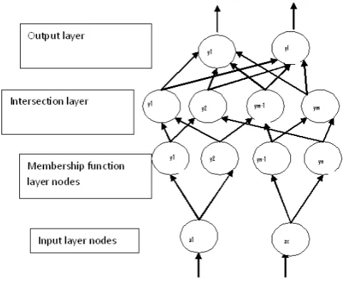
Let be our network has number of inputs, like (a1, a2, a3…., ax) and classes (c1, c1…, cc). The first layer is the input layer, the second layer is the membership function and feature selection layer, the third layer is called the intersection layer [1] and the fourth layer is the output layer. The activation function of each node with its inputs and outputs are discussed next layer by layer.
Layer 1: The number of nodes in this layer is equal to x. Let ap be the input to the pth node in layer 1 then the
output of this section is
yp= ap (1)
Layer 2: Each node in this layer represents the membership function of a linguistic value associated with an input linguistic variable. The output of a layer 2 node represents the membership grade of the input with respect to a linguistic value. Bell shaped membership functions are used here. All connection weights between the
nodes in layer 1 and layer 2 are unity. If there be Si fuzzy sets associated with the ith feature then the number of
nodes in this layer is Σi-1s Si. The output of a node in layer 2 is computed by
yn=exp{-(yp-µn)2/σn2} (2)
µnand σnare the centre and spread, respectively [8] of the bell shaped function. The tuneable parameter
βpassociated with each input feature ap called a feature modulator.βps are learned by back-propagation
2
- βp
yn = y (1-e ) (3)
When βp takes a large value then yn tends to yn and for small values of βp2 , yn tends to 1, thereby making the
feature indifferent. In learning phase I, the parameters of the membership functions are kept fixed and only the
βps are learned through error back-propagation. In learning phase III, the βps is kept fixed and the membership
function parameters are updated.
Fig .1.The Network Structure
Layer 3: This layer is called the antecedent layer. Each node in this layer represents the IF part of a fuzzy
rule.Number of nodes in layer 3 is 81. The output of the mth node in layer 3 is 1/q
∑ nεPmyqn
ym = (4) |Pm|
Layer 4: The nodes in this layer perform an OR operation, which combines the intersection node of layer 3 with layer 4. The output of node in this layer represents the certainty with which a data point belongs to class l
yl= maxnεPm ( ymωlm ) (5)
where pl represents the set of indexes of the nodes in layer 3 connected to the node l of layer 4. Since ωlm s are
interpreted as certainty factors, each should be non-negative and it should lie in [0, 1]. The error
back-propagation algorithm or any other gradient based search algorithm does not guarantee that ωlm will remain
non-negative, even if one starts the training with non-negative weights [1] and hence, the model ωlm by e-glm2 . The
non- negative alone would be enough. So ωlm = glm2 Therefore, the output (activation function) of the lth node in
layer 4 will be
yl = maxmεPl(ymg2lm) (6)
Learnable weights ωlm are updated in all the three learning phases.
3. ERROR ANALYSIS
Error back-propagation algorithm is used for error analysis. The simple perception is just able to handle linearly separable or linearly independent problems. By taking the derivative of the error of the network with respect to each weight, [9] one will learn a little about the direction of the error. In fact, if one takes the negative of this derivative and then proceeds to add it to the weight, the error will decrease until it reaches local minima.
This makes sense because if the derivative is positive, it indicates that the error is increasing when the weight is increasing. The obvious thing to do then is to add a negative value to the weight and vice versa if the derivative is negative. Because the taking of these partial derivatives and then applying them to each of the weights takes place, starting from the output layer to hidden layer weights, then the hidden layer to input layer
weights. This algorithm has been called the error back-propagation algorithm. All the training phases use the
concept of back-propagation to minimize the error function N N c
Layer 4: The output of nodes in this layer əE
Δ1= əzl
Thus
Δl=-(ol-yl) (8)
Layer 3: Δm of this layer will be
Δm=əE/əym
Then the output of Δm will be
Δm = (∑lεQm Δl glm2) (9)
Here Q m is the set of indexes of the nodes in layer 4 connected with node m of layer 3.
Layer 2: Δn for layer 2 is
Δn = əE/əyn
Hence,
ym ynq-1
Δn = ∑ Δm (10)
mεRn ΣnεPm ynq
Rn is the set of indexes of nodes in layer 3 connected with node n in layer 2.
With the Δ calculated for each layer now we can write the weight update equation and the equation
for updating βp.
əE/ə glm = ( əE/əzl )(əzl/ə glm ) (11)
e=1/2∑Ei =1/2 ∑∑(oil –yil )2 (7)
The delta value Δ of a node in the network is defined as the influence of the node output on E The derivation of the delta values and adjustment of the weights are presented by layer wise next.
əE/ə glm = (∑lεQm 2Δlzm glm). (12)
Similarly
əE/əβp = -∑Δn (2 βp e-βp2 y n) (yp -µn 2) (13)
nεRp σn
Hence the update equations for weights glm and βp
glm (t+1) = glm (t) – (0.01* əE/əglm) (14)
βp (t+1) = βp (t) – (0.01* əE/əβp ) (15)
Update of these values will reduce the error
4. TUNING OF MEMBERSHIP FUNCTION
While the tuning of membership function parameters tries to improve the performance of a rule, tune parameters of the membership functions considering each rule separately. As a result, if both modulator functions and membership function parameters [2] are tuned, the learning process may become unstable. Therefore, tuning of parameters of membership functions should be done after feature elimination.
Table.1.Summary of data sets.
5. RESULT AND DISCUSSION
Iris flower has four features and three classes Here we have used three fuzzy set for each of the four features.
In this case the initial network has 81 intersection nodes resulting in 81*3=243 rules. After pruning of the redundant nodes the number of intersection nodes becomes 9, hence, at this stage the number of rules is
9*3=27 rules. Next, the incompatible rules are pruned to obtain nine rules. For IRIS flower we found four less
used rules and we removed them. The final architecture represented only five rules that are depicted in Figure 1.
Name Total
size
Test size
No. Of classes
No. Of features
Fig.2.Rules for classification of iris
Linguistic rules are shown in Table .2. In IRIS data features 3 and 4 represent petal length and petal width of iris flower, respectively. In Table 3 pl and pw represent the petal length and petal width, respectively.
Table.2.Initial Architecture of the Network used for IRIS
Layer 1 3
Layer 2 12
Layer 3 81
Layer 4 3
In Table 3 pl and pw represent the petal length and petal width, respectively.
Table.3. Rules for IRIS Data length and petal width of iris flower
Rule No Rule Class
1 If pl is close to 1.5 & pw is close to
0.25
Class 1
2 If pl is close to 4.5 & pw is close to
1.25
Class 2
3 If pl is close to 6.5 & pw is close to
1.25
Class 3
4 If pl is close to 4.5 & pw is close to
2.25
Class 3
5 If pl is close to 6.5 & pw is close to
2.25
Pruning of redundant nodes reduces the number of intersection classes to 81. The removal of incompatible rules
consequently yields 81 rules. Among these 81 rules 32 rules were zero rulesand there were no less used rules.
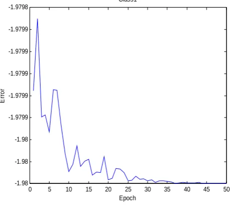
Result of error with epoch shown in figure 3for class1, figure 4 for class 2, and figure 5 for class 3.
0 5 10 15 20 25 30 35 40 45 50
-1.98 -1.98 -1.98 -1.9799 -1.9799 -1.9799 -1.9799 -1.9799 -1.9798
E
rro
r
Epoch Class1
Fig.3. Error approach for class 1
Error is minimized after 30 epochs itself .Error is calculated by error back-propagation.
0 5 10 15 20 25 30 35 40 45 50
-1.98 -1.98 -1.98 -1.98 -1.98 -1.98 -1.98 -1.98 -1.98 -1.98
E
rro
r
Epoch Class2
Fig . 4. Error approach for class2
0 5 10 15 20 25 30 35 40 45 50 -1.98
-1.98 -1.98 -1.98 -1.98 -1.98 -1.98 -1.98 -1.98
Er
ro
r
Epoch Class3
Fig.5.Error approach for class 3
5. CONCLUSION
A fuzzy modelling tool for target selection in direct marketing has been developed. Here the network starts with all possible rules and the training process retains only the rules required for classification, thus resulting in a smaller architecture of the final network. The final network has a lower running time than the initial network. The error result between the training and test sets were obtained.Important problem of interest related to this may be to find the sensitivity of the output of a neuro-fuzzy classifier with respect to its internal parameters. Therefore, authors believe that this architecture is general enough for use in other rule-based systems which perform fuzzy logic inference.
REFERENCES
[1] Barenji H.R and Khedkar,P, , “Learning and tuning fuzzy controllers through reinforcements”, IEEE Trans. Neural Networks, vol. 3, pp. 724-740, 1992.
[2] Chakraborty. D and Pal. N. R, “Integrated feature analysis and fuzzy rule-based system identification in a neuro-fuzzy paradigm”, IEEE Trans. Syst. Man Cybern. B, vol. 31, pp. 391–400. , 2001.
[3] Chakraborty.D and Pal.N.R, ,”Neuro-Fuzzy Scheme for Simultaneous Feature Selection and Fuzzy Rule-Based Classification”, IEEE Trans. Neural Networks, Vol.15, pp.110-123,2001.
[4] Freeman.J.A and Skapura.B.M, , “Neural networks, Algorithms applications and programming Techniques”,Addison-Wesely,1990. [5] Ishibuchi. H and Nozaki .K, Yamamoto .N, and Tanaka. H, “Selecting fuzzy if-then rules for classification problems using genetic
algorithms”, IEEE Trans. Fuzzy Syst., vol. 3, pp.260–27,1990.
[6] Kasabov .Nand Song .Q, “DENFIS: dynamic evolving neural-fuzzy inference system and its application for time series prediction”, IEEE Trans. Fuzzy Syst., vol. 10, pp.144-154,2002.
[7] Mao. J and Jain A. K, “Artificial neural networks for feature extraction and multivariate data projection”, IEEE Trans. Neural Networks, vol. 6, pp.296–317, 1995.
[8] Sandeep Paul and Satish Kumar, “Subsethood-Product Fuzzy Neural Inference System (SuPFuNIS)”, IEEE Trans.Neural Networks,Vol.13, pp.578-599,2002.
[9] Sathish Kumar, “Neural Networks: A Classroom Approach”, Tata McGraw-Hill Publishing Company, New Delhi, 2004.
[10] Setnes .M and Kaymak. U, “Fuzzy modelling of client preference from large data sets: an application to target selection in direct marketing”, IEEE Trans. Fuzzy Syst., vol. 9, pp. 153–163, 2001.