University of Pennsylvania
ScholarlyCommons
Publicly Accessible Penn Dissertations
1-1-2014
Learning, Large Scale Inference, and Temporal
Modeling of Determinantal Point Processes
Raja Mohd Hafiz Affandi Raja Ahmad
University of Pennsylvania, [email protected]
Follow this and additional works at:http://repository.upenn.edu/edissertations
Part of theComputer Sciences Commons, and theStatistics and Probability Commons
This paper is posted at ScholarlyCommons.http://repository.upenn.edu/edissertations/1411
Recommended Citation
Raja Ahmad, Raja Mohd Hafiz Affandi, "Learning, Large Scale Inference, and Temporal Modeling of Determinantal Point Processes" (2014).Publicly Accessible Penn Dissertations. 1411.
Learning, Large Scale Inference, and Temporal Modeling of Determinantal
Point Processes
Abstract
Determinantal Point Processes (DPPs) are random point processes well-suited for modelling repulsion. In discrete settings, DPPs are a natural model for subset selection problems where diversity is desired. For example, they can be used to select relevant but diverse sets of text or image search results. Among many remarkable properties, they offer tractable algorithms for exact inference, including computing marginals, computing certain conditional probabilities, and sampling.
In this thesis, we provide four main contributions that enable DPPs to be used in more general settings. First, we develop algorithms to sample from approximate discrete DPPs in settings where we need to select a diverse subset from a large amount of items.
Second, we extend this idea to continuous spaces where we develop approximate algorithms to sample from continuous DPPs, yielding a method to select point configurations that tend to be overly-dispersed.
Our third contribution is in developing robust algorithms to learn the parameters of the DPP kernels, which is previously thought to be a difficult, open problem.
Finally, we develop a temporal extension for discrete DPPs, where we model sequences of subsets that are not only marginally diverse but also diverse across time.
Degree Type Dissertation
Degree Name
Doctor of Philosophy (PhD)
Graduate Group Statistics
First Advisor Eric T. Bradlow
Keywords
Determinantal Point Processes, diversity, large-scale, learning, point processes, repulsion
Subject Categories
LEARNING, LARGE SCALE INFERENCE, AND TEMPORAL
MODELING OF DETERMINANTAL POINT PROCESSES
Raja Mohd Hafiz Affandi Raja Ahmad
A DISSERTATION
in
Statistics
For the Graduate Group in Managerial Science and Applied
Economics
Presented to the Faculties of the University of Pennsylvania
in
Partial Fulfillment of the Requirements for the Degree of Doctor of
Philosophy
2014
Supervisor of Dissertation
Eric Bradlow, K.P. Chao Professor, Marketing, Statistics and
Education
Graduate Group Chairperson
Eric Bradlow, K.P. Chao Professor, Marketing, Statistics and
Education
Dissertation Committee
LEARNING, LARGE SCALE INFERENCE, AND TEMPORAL
MODELING OF DETERMINANTAL POINT PROCESSES
COPYRIGHT
2014
Raja Mohd Hafiz Affandi Raja Ahmad
This work is licensed under the Creative Commons
Attribution-NonCommercial-ShareAlike 3.0 License
To view a copy of this license, visit
Acknowledgments
In the name of God, the Most Gracious, the Most Merciful. My highest gratitude
goes my Lord for His blessing and everything that I have.
My first debt of appreciation must go to my advisor, Emily Fox, for her endless
encouragement and guidance without which this work would not have been possible.
She is undoubtedly a great mentor and is someone who I look up to throughout
my years as her student. This thesis is written in the memory of Ben Taskar,
who was not only the smartest person I’ve known but also possessed a gentle and
loving heart. His guidance, patience and kindness will always be remembered. To
Alessandro Rinaldo, who was the first to pique my interests in statistics– without
you, I wouldn’t have even started this journey towards my Ph.D. I would also like
to thank my committee members, Eric Bradlow, Dean Foster and Sasha Rakhlin
for their valuable advice, helpful suggestions and constructive criticisms in finishing
this thesis.
I am forever indebted to the friendship and constant love and support from my
family and friends. First and foremost, this thesis is dedicated to my late mother,
Raja Hafizah Raja Khalid, whose neverending love made me strive to be the best
that I can. To my father, Raja Ahmad Raja Shah Kobat– my deepest love for
never giving up on me even when at times it seems that I’m stumbling through
life. To my sisters and brother, Mimi (Ayong), Elina (Angah) and Kamil (Abang),
and uncle, Raja Hamizah and Zairi, words cannot express how indebted I am to
you for treating me like your own son. To my fianc´ee, Ada– I honestly don’t think
I could have finished this thesis without you. You are such an inspiration in my
ABSTRACT
LEARNING, LARGE SCALE INFERENCE, AND
TEMPORAL MODELING OF DETERMINANTAL
POINT PROCESSES
Raja Mohd Hafiz Affandi Raja Ahmad
Eric Bradlow
Determinantal Point Processes (DPPs) are random point processes well-suited
for modelling repulsion. In discrete settings, DPPs are a natural model for subset
selection problems where diversity is desired. For example, they can be used
to select relevant but diverse sets of text or image search results. Among many
remarkable properties, they offer tractable algorithms for exact inference, including
computing marginals, computing certain conditional probabilities, and sampling.
In this thesis, we provide four main contributions that enable DPPs to be used
in more general settings. First, we develop algorithms to sample from approximate
discrete DPPs in settings where we need to select a diverse subset from a large
amount of items.
Second, we extend this idea to continuous spaces where we develop approximate
algorithms to sample from continuous DPPs, yielding a method to select point
configurations that tend to be overly-dispersed.
Our third contribution is in developing robust algorithms to learn the parameters
of the DPP kernels, which is previously thought to be a difficult, open problem.
Finally, we develop a temporal extension for discrete DPPs, where we model
sequences of subsets that are not only marginally diverse but also diverse across
Contents
Acknowledgments . . . iv
List of Tables . . . x
List of Figures . . . xii
1 Introduction 1 1.1 Contributions . . . 4
1.2 Thesis Outline . . . 5
2 Background 7 2.1 Discrete DPPs . . . 7
2.1.1 Marginals and Conditionals . . . 9
2.1.2 Sampling Discrete DPPs . . . 10
2.1.3 Fixed-sized kDPPs . . . 11
2.1.4 Quality-Similarity Decomposition . . . 13
2.1.5 Dual Representation of DPPs . . . 14
2.1.6 Learning Discrete DPPs . . . 14
2.2 Continuous DPPs . . . 17
2.2.1 Example of Continuous Kernels . . . 19
2.2.2 Sampling from a Continuous DPPs . . . 21
2.2.3 Learning Continuous DPPs . . . 22
2.3 Low-Rank Kernel Approximations . . . 23
2.3.1 Nystr¨om Approximation . . . 23
2.3.2 Random Fourier Features . . . 25
2.4 Markov-Chain Monte Carlo (MCMC) . . . 26
2.4.1 Metropolis-Hastings (MH) . . . 27
2.4.2 Slice Sampling . . . 28
3 Large-Scale Inference of Discrete DPPs 32 3.1 Low-Rank Approximated DPPs/kDPPs . . . 34
3.1.1 Preliminaries . . . 37
3.1.2 Set-wise bounds for DPPs . . . 38
3.1.4 Nystr¨om-approximated DPPs . . . 43
3.1.5 RFF-approximated DPPs . . . 46
3.2 Experiments . . . 48
3.3 Conclusion . . . 51
4 Inference for Continuous DPPs 54 4.1 Sampling from a Low-Rank Continuous DPP . . . 57
4.1.1 Sampling from a Nystr¨om-approximated DPP . . . 61
4.1.2 Sampling from an RFF-approximated DPP . . . 64
4.2 Gibbs Sampling . . . 66
4.3 Analysis . . . 69
4.3.1 Analysis of Low-Rank Approximation Sampling . . . 69
4.3.2 Empirical Study of Low-Rank Approximation Sampling . . . 71
4.3.3 Empirical Study of Gibbs Sampling . . . 73
4.4 Experiments . . . 76
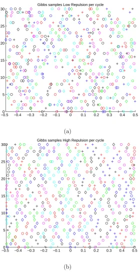
4.4.1 Repulsive priors for mixture models . . . 76
4.4.2 Latent clustering of social networks . . . 85
4.4.3 Generating diverse sample perturbations . . . 88
4.5 Conclusion . . . 91
5 Large-Scale Learning of DPPs 93 5.1 Learning Parametric DPPs . . . 94
5.1.1 Learning using Optimization Methods . . . 95
5.1.2 Bayesian Learning for Discrete DPPs . . . 99
5.1.3 Bayesian Learning for Large-Scale Discrete and Continuous DPPs . . . 101
5.2 Method of Moments . . . 111
5.3 Experiments . . . 114
5.3.1 Simulations . . . 114
5.3.2 Diabetic Neuropathy . . . 116
5.3.3 Diversity in Images . . . 120
5.3.4 Learning Mixture Model Parameters . . . 124
5.4 Conclusion . . . 126
6 Markov DPPs 127 6.1 Markov DPPs (M-DPPs) . . . 130
6.1.1 First Order M-DPPs . . . 131
6.1.2 First Order MarkovkDPPs . . . 135
6.1.3 Sampling from First Order M-DPPs and M-kDPPs . . . 137
6.1.4 Higher Order M-DPPs . . . 138
6.1.5 Higher Order M-kDPP . . . 143
6.1.6 Sampling from Higher Order M-DPPs and M-kDPPs . . . . 144
6.2 Learning User Preferences . . . 145
6.2.2 Likelihood Based Alternatives . . . 150
6.3 Experiments . . . 151
6.3.1 Fixed Quality . . . 151
6.3.2 Learning Preferences . . . 154
6.4 Conclusion . . . 160
7 Conclusion 162 7.1 Future Work . . . 163
List of Tables
3.1 Results for user study on MoCap summarization. . . 53
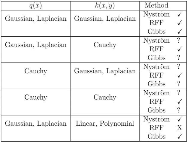
4.1 Examination of the feasibility of DPP sampling using Nystr¨om, RFF approximations and Gibbs sampling. . . 56
4.2 Comparison between Gibbs and Nystr¨om-approximated DPP samples 76
4.3 Quantitative comparison betweenIID and DPPmodels. . . 84
4.4 Classification errorIIDand DPP. . . 85
4.5 Misclassification rates for Monk Data . . . 88
5.1 Examination of the feasibility of learning the parameters of DPP kernels using gradient-based methods. . . 98 5.2 Examination of the feasibility of sampling from exact posteriors of
the parameters of DPP kernels using MCMC-based methods. . . 111
List of Figures
2.1 Comparing DPP and Poisson point process samples on a 2-D plane. 9
2.2 Sampling DPP over two-dimensional grid positions . . . 12
2.3 Univariate slice sampling. . . 30
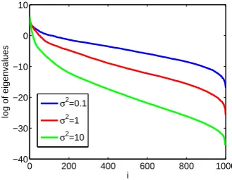
3.1 Log-eigenvalues for MNIST, Abalone and synthetic datasets. . . 44
3.2 Error of Nystr¨om approximations. . . 45
3.3 Comparison between errors of Nystr¨om and random Fourier features approximations . . . 47
3.4 The log-eigenvalues of RBF kernel applied to the Abalone datset. . 47
3.5 Sample screen from the user study for the MoCap summarization experiment. . . 51
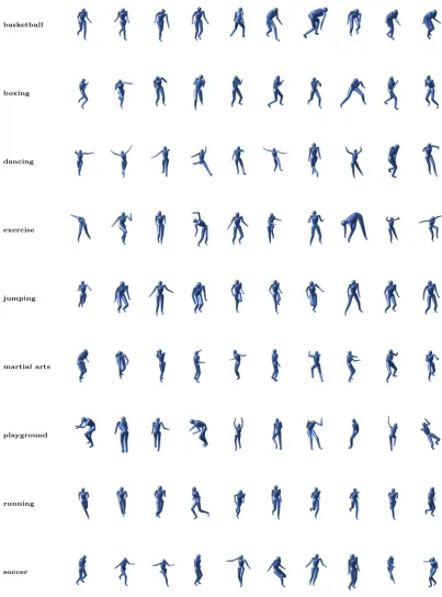
3.6 DPP samples for each activity in the MoCap videos. . . 52
3.7 Comparison between MoCap video frames chosen randomly and frames sampled from the Nystr¨om-approximated DPP. . . 53
4.1 Estimates of total variational distance for Nystr¨om and RFF- ap-proximated DPPs . . . 72
4.2 Plots of location of DPP samples using Gibbs scheme. . . 75
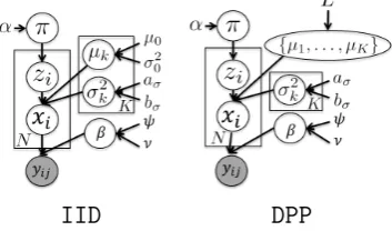
4.3 Graphical models for mixtures of Gaussians usingIIDandDPPpriors on the location parameters. . . 77
4.4 Comparison between the full conditional for µk using the IIDand DPPmodels. . . 81
4.5 Qualitative comparison between IID and DPPmodels. . . 83
4.6 Graphical models for latent clustering of social network usingIID and DPPpriors on the location parameters. . . 86
4.7 Social network clustering on Monk data with 3 clusters. . . 87
4.8 Social network clustering on Monk data with 5 clusters. . . 88
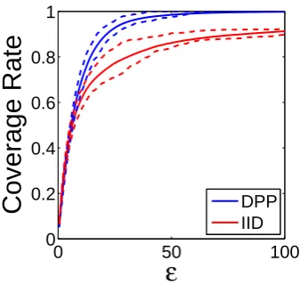
4.9 Fraction of MoCap data having a DPP/i.i.d. sample within an -neighborhood. . . 90
4.10 Comparison between principal components of DPP and i.i.d samples fromdance data. . . 90
5.1 Sample autocorrelation function for posterior samples obtained using MH and slice sampling. . . 101 5.2 Slice sampling algorithm using posterior bounds. . . 104 5.3 Normalizer bounds for a discrete Gaussian DPP. . . 108 5.4 Posterior samples for a continuous DPP with Gaussian quality and
similarity. . . 116 5.5 Moment estimates under the parameters learned for a continuous
DPP with Gaussian quality and similarity. . . 117 5.6 Nerve fiber samples. . . 118 5.7 The repulsion measure,γ under the two learned DPP classes. . . . 119 5.8 The leave-one out log-likelihood of each sample under the two learned
DPP classes. . . 120 5.9 Boxplots of posterior samples for the image diversity experiment. . 125
6.1 Sequence of samples drawn independently from a DPP. . . 128 6.2 Sequence of samples drawn from a first order Markov-DPP. . . 129
6.3 Sequence of samples drawn from a second order Markov-DPP. . . . 129
6.4 Comparison between sets of points on a line drawn using independent DPP and using Markov-DPP. . . 130 6.5 Drawing a thinned−kDPP sample. . . 136 6.6 Performance of the methods at recovering the preselected preferred
articles. . . 154 6.7 Cumulative fraction of preferred articles displayed to the user. . . . 156 6.8 Headlines selected on days 99 (left) and 100 (right). . . 158 6.9 The fraction of preferred articles displayed to user at each time step
Chapter 1
Introduction
A determinantal point process (DPP) provides a distribution over configurations
of points. The defining characteristic of the DPP is that it is a repulsive point
process, which makes it useful for modeling diversity. DPPs were first identified
as a class by Macchi [1975] who used them to model the distributions of fermion
systems at thermal equilibrium. Since the Pauli exclusion principle states that
no two fermions can occupy the same quantum state, this repulsiveness is aptly
described by a DPP.
Formally, given a space Ω ⊆Rd, a specific point configuration A⊆Ω, and a
positive semi-definite kernel functionL: Ω×Ω→R, the probability density under
a DPP with kernelL is given by
PL(A)∝det(LA) , (1.1)
where LA is the |A| × |A| matrix with entries L(x,y) for each x,y∈A. This
defines a repulsive point process since point configurations that are more spread
out according to the metric defined by the kernel L have higher densities. To see
then the subdeterminant in Eq. (1.1) is proportional to the square of the volume
spanned by the kernel vectors associated with the points inA.
Despite the interesting repulsive characteristic they present, DPPs did not
receive much attention beyond the community of mathematical physics and
proba-bility for a few decades. This changed in the mid-to-late 2000s, when it was found
that DPPs in discrete spaces yield appealing mathematical properties including
computation of marginal and conditional probabilities [Borodin and Rains, 2005,
Borodin, 2009] and efficient sampling algorithms [Hough et al., 2006].
With the advent of the theory in discrete settings, DPPs have recently played
an increasingly important role in machine learning and statistics. With discrete
DPPs’ growing recognition as a method for diverse subset collection, they have
been widely applied to tasks such as pose estimation [Kulesza and Taskar, 2010],
image search [Kulesza and Taskar, 2011a], news thread discovery [Gillenwater et al.,
2012] and neural spiking models [Snoek et al., 2013].
For discrete DPPs, there exists a sampling algorithm that is exact and efficient
[Hough et al., 2006]. Given N base points (or items), {x1, . . . ,xN}= Ω, sampling
can be done using an eigendecomposition of the DPP kernel matrix L and it runs
in time O(N3) despite sampling from a distribution over 2N subsets. However,
when N is very large, anO(N3) algorithm can be prohibitively slow; for instance,
when selecting a subset of frames to summarize a long video. Furthermore, while
storing a vector ofN items might be feasible, storing an N×N matrix often is not.
The first contribution of this thesis is then to provide an approximate algorithm
to sample from large-scale DPPs using low-rank approximations of the kernel
matrix. While many low-rank approximation algorithms exist with guaranteed
performance in terms of the matrix norm, it is not clear how the errors propagate
provide bounds on the error of DPPs based on low-rank approximated kernels.
Our algorithm will provide a method for diverse subset sampling in large-scale
settings. For example, we will consider the application to motion capture video
summarization.
DPPs defined on continuous spaces have also been found useful in applications
such as repulsive mixture modeling [Zou and Adams, 2012] where generating point
configurations that tend to be spread out is desirable. However, the use of DPPs
are somewhat limited due to the lack of efficient sampling algorithms. Our second
main contribution is this thesis is to propose an efficient algorithm to sample from
DPPs in continuous spaces using low-rank approximations of the kernel function.
We investigate two such schemes: Nystr¨om and random Fourier features. Our
approach utilizes a dual representation of the DPP, a technique that has proven
useful in the discrete Ω setting as well [Kulesza and Taskar, 2010]. For k-DPPs,
which only place positive probability on sets of cardinality k [Kulesza and Taskar,
2012a], we also devise a Gibbs sampler that iteratively samples points in the k-set
conditioned on all k−1 other points. The derivation relies on representing the
conditional DPPs using the Schur complement of the kernel. As a result, our
methods allow for the sampling of repulsive point configurations in continuous
spaces. We consider their applications to repulsive Gaussian mixture models and
synthesis of human motion.
Despite many remarkably efficient algorithms for inference of DPPs, an
impor-tant component of DPP modeling — learning the DPP kernel parameters — is
still considered a difficult, open problem. Even in the discrete Ω setting, DPP
kernel learning has been conjectured to be NP-hard [Kulesza and Taskar, 2012a].
Intuitively, the issue arises from the fact that in seeking to maximize the
the normalizer contributes a convex term, leading to a non-convex objective. This
non-convexity holds even under various simplifying assumptions on the form of L.
Our third main contribution in this thesis is to provide robust algorithms to learn
the parameters of the DPP kernel. We propose Bayesian methods to learn the DPP
kernel parameters. These methods can be used to efficiently learn both discrete
and continuous DPPs, even in cases where gradient-based optimization methods
are not even feasible. We provide applications to classifying nerve fiber data in
diabetic patients and human judgement of image diversity.
Finally, we present a temporal extension to discrete DPPs, where we model
diverse sequences of subsets. In many applications, it is desirable to select subsets
that are not only marginally diverse but also diverse relative to those previously
shown. For example, in displaying news headlines from day-to-day, one aims to
select articles that are relevant and diverse on any given day and also diverse to
the articles that are shown in the previous days. We construct a Markov DPP
(M-DPP) for a sequence of random sets that defines a stationary process that
maintains DPP margins, implying that the subset chosen is encouraged to be
diverse at a particular time t. Crucially, the union of consecutive subsets is also
marginally DPP-distributed implying diversity across time as well. We will consider
the application of M-DPP in displaying daily news headline.
We believe this thesis will open up opportunities to use DPPs as parts of many
models, both in discrete and continuous settings, as well as spur further research
in developing theoretical properties and efficient algorithms for general classes of
DPPs.
1.1
Contributions
• We provide an approximate algorithm to sample from large-scale DPPs using
low-rank approximations of the kernel matrix. We provide bounds on the
error of DPPs based on these low-rank approximated kernels.
• We propose propose an efficient algorithm to sample from DPPs in continuous
spaces using low-rank approximations of the kernel function. We provide
bounds on the error of DPPs based on these low-rank approximations. For
fixed-sized k-DPPs, we also devise a Gibbs sampler that iteratively samples
points in thek-set conditioned on all k−1 other points.
• We provide robust algorithms to learn the parameters of the DPP kernel
using Bayesian methods. These methods can be extended to efficiently learn
large-scale discrete and continuous DPPs.
• We present a temporal extension to discrete DPPs, where we model diverse
sequences of subsets. Our construction defines a stationary process that
maintains DPP margins, implying that the subset chosen is encouraged to be
not only diverse at a particular time t but the union of consecutive subsets
are also marginally DPP-distributed implying diversity across time as well.
• We provide a variety of experimental results along the way, demonstrating
the successful application of our methods to real-world tasks including video
summarization, repulsive mixture model, repulsive social network clustering,
human motion synthesis, diabetic neuropathy classification, human judgement
of image diversity and news retrieval.
1.2
Thesis Outline
• Chapter 2: BackgroundWe present a survey of DPPs including existing
sampling and learning algorithms. We will also present a number of
well-known low-rank approximation methods and MCMC-based algorithms which
we will heavily rely on in sampling and learning large-scale/continuous DPPs.
• Chapter 3: Large-Scale Inference of Discrete DPPs We provide our
approximate sampling algorithm for large-scale discrete DPPs along with
error bounds associated with our methods and an empirical study of these
bounds, along with applications to motion capture video summarization.
• Chapter 4: Inference of Continuous DPPs We extend the sampling
algorithm to the continuous case in addition to a Gibbs sampling-type
algorithm for fixed-sized DPPs and apply them to repulsive Gaussian mixture
models and synthesis of human motion.
• Chapter 5: Large-Scale Learning of DPPs: We propose Bayesian
algorithms to learn kernel parameters of DPPs. We show how MCMC-type
algorithms can be modified to enable efficient learning of large-scale discrete
and continuous DPPs, even when likelihoods cannot be exactly or efficiently
computed but can be bounded instead. We provide applications to classifying
nerve fiver data in diabetic patients and human judgement of image diversity.
• Chapter 6: Markov DPPs We present our construction of Markov DPPs
that defines a stationary process that maintains individual diversity as well
as diversity across time. We provide their applications to displaying daily
news headline.
• Chapter 7: ConclusionWe summarize our contributions and discuss their
Chapter 2
Background
In this chapter, we first present a survey of DPPs. We provide a definition of
DPPs in discrete spaces and its interpretation and explore existing sampling and
learning algorithms. We then present the extension of DPPs to continuous spaces.
Finally, we present a number of well-known low-rank approximation methods and
MCMC-based algorithms which we will heavily rely on in sampling and learning
large-scale/continuous DPPs.
2.1
Discrete DPPs
A random point process P on a discrete base set Ω ={x1,x2, . . . ,xN} is a
proba-bility measure on the set 2Ω of all subsets of Ω. P is called a determinantal point
process (DPP) if there exists a positive semidefinite matrix L indexed by elements
of Ω such that the probability of sampling a setA ⊆Ω is given by [Borodin and
Rains, 2005]:
PL(A) =
det(LA)
LA≡[Lij]xi,xj∈A is the submatrix of L indexed by the elements inA and I is the
N ×N identity matrix. Here we adopt the convention that det(L∅) = 1. This
representation of DPPs is known as the L-ensemble [Borodin and Rains, 2005].
The subdeterminant in Eq. (2.1) has an intuitive geometric interpretation. If
we let B be a D×N matrix such thatL=B>B, then if we denote the columns
of B byBi, i= 1,2, . . . , N, we get the following expression:
det(LA) = Vol2({Bi}xi∈A) (2.2)
where the right hand side denotes the square |A|-dimensional volume of the
parallelepiped spanned by the columns of B corresponding to the elements in
A. For this reason, DPPs give high probability to subsets that are diverse since
they are more orthogonal (and hence span larger volumes). Fig. 2.1 shows the
difference between sampling a set of points in the plane using a DPP (with Lij
inversely related to the distance between points xi andxj) and sampling points
independently. While the latter results in random clumping of the points, DPP
sampling, on the other hand, leads to a relatively uniformly spread set with good
coverage.
Due to the fact that DPPs favor selecting subsets that are diverse, they have
played an importand role in many machine learning tasks such as pose estimation
[Kulesza and Taskar, 2010], image search [Kulesza and Taskar, 2011a], salient news
thread discovery [Gillenwater et al., 2012] and neural spiking [Snoek et al., 2013]
where getting a good coverage of items is key. Coupled with appealing mathematical
properties and efficient algorithms explored in the next few subsections, discrete
Figure 2.1: A set of points in the plane drawn from a DPP (left), and the same number of points sampled independently using a Poisson point process (right). This figure is taken from Kulesza and Taskar [2012a].
2.1.1
Marginals and Conditionals
Marginals A DPP can also be represented in terms of its marginal kernel. Let
K be a semidefinite matrix such that K I (all eigenvalues less than or equal to
1). Then ifY is a random set drawn according to the DPP with marginal kernel
K, then for every A⊆Ω:
P(Y ⊇A) = det(KA) . (2.3)
Once again, KA≡[KA]xi,xj∈A denotes the submatrix of K indexed by elements in
A, and we adopt the convention that det(K∅) = 1. If we think of Kij as measuring
the similarity between items i and j, then
P(Y ⊇ {xi,xj}) =KiiKjj −Kij2 (2.4)
implies that Y is unlikely to contain both xi and xj when they are very similar.
Here as well, a DPP can be seen as modeling a collection of diverse items from the
K = L(I+L)−1 =I−(L+I)−1 [Macchi, 1975]. Conversely, a DPP with marginal
kernel K has L-ensemble kernelL=K(I−K)−1 (when the inverse exists).
Conditionals For any A, B ⊆ Y with A∩B =∅, it can be shown that [Kulesza
and Taskar, 2012a]
PL(Y =A∪B|Y ⊇A) =
det(LA∪B)
det(L+IΩ\A)
, (2.5)
where IΩ\A is a matrix with ones on the diagonal entries indexed by the elements
of Ω\A and zeros elsewhere.
This conditional distribution is itself a DPP over the elements of Ω\A [Borodin
and Rains, 2005]. In particular, supposeY is DPP-distributed with L-ensemble
kernel L, and condition on the fact that Y ⊇ A. Then the set Y \A is
DPP-distributed with marginal and L-ensemble kernels
KA =
I−(L+IΩ\A)−1
Ω\A (2.6)
LA =(L+IΩ\A)−1
Ω\A
−1
−I . (2.7)
Here, [·]Ω\A denotes the submatrix of the argument indexed by elements in Ω\A.
Thus, DPPs as a class are closed under most natural conditioning operations.
2.1.2
Sampling Discrete DPPs
Hough et al. [2006] first described the DPP sampling algorithm shown in
Algo-rithm 1. Phase 1 is to compute an eigendecomposition L=PN
n=1λnvnvn> of the
kernel matrix; from this, a random subset V of the eigenvectors is chosen by using
the eigenvalues to bias a sequence of coin flips. The Phase 2 of algorithm proceeds
Algorithm 1 Sampling discrete DPPs
Input: L-ensemble kernel matrix L
{(vn, λn)}Nn=1 ← eigenvector/value pairs of L
J ← ∅
for n= 1, . . . , N do
J ←J ∪ {n} with prob. λn
λn+1
V ← {vn}n∈J
Y ← ∅
while |V|>0 do
Select yi from Ω with Pr(yi)= |V1|Pv∈V(v
>e
i)2
Y ←Y ∪ {yi}
V ←V⊥, an orthonormal basis for the subspace of V orthogonal to ei
Output: Y
updating V in a manner that de-emphasizes items similar to the one just selected.
Note that ei is the ith elementary basis vector whose elements are all zero except
for a one in position i. Alg. 1 runs in time O(N3+N k3), where N is the number
of available items and k is the cardinality of the returned sample.
The sampling algorithm has an intuitive interpretation. The initial sampling of
a point is proportional to the square of the projection of the points to the collection
of selected eigenvectors. Thus points that align closer to the eigenvectors have a
higher probability of being chosen. However, as each successive point is selected
andV is updated by Gram-Schmidt orthogonalization, the distribution shifts to
avoid points near those already chosen. Fig. 2.2 shows a progression for a DPP
sampling over points in the unit square.
2.1.3
Fixed-sized
k
DPPs
In selecting a diverse collection of elements in Ω, a DPP jointly models both the
size of a set and its content. In some applications, the goal is to select (diverse) sets
of a fixed size. In order to achieve this goal, we can instead consider a fixed-size
Figure 2.2: Sampling DPP over two-dimensional grid positions. Red circles indicate already selected positions. On the bottom,lighter color corresponds to higher probability. The DPP naturally reduces the probabilities for positions that are similar to those already selected. This figure is taken from Kulesza and Taskar [2012a].
a distribution over all random subsets Y ⊆ Ω with fixed cardinality k. The
L-ensemble construction of a kDPP, denoted PLk, gives probabilities
Pk
L(Y =A) =
det(LA) P
|B|=kdet(LB)
(2.8)
for all sets A with cardinality k and any positive semidefinite kernel L. While
the normalization constant cannot expressed as conveniently as the regular DPP,
Kulesza and Taskar [2011a] show that the kDPP distribution can be written as
Pk L(A) =
det(LA)
ek(λ1, . . . , λN)
Algorithm 2 Sampling from a kDPP
Input: L-ensemble kernel matrix L, size k
{(vn, λn)}Nn=1 ← eigenvector/value pairs of L
J ← ∅
for n=N, . . . ,1 do
if u∼U[0,1]< λn
enk−−11 enk then
J ←J∪ {n}
k←k−1
if k = 0 then break
{continue with the rest of Algorithm 1}
where λ1, . . . , λN are eigenvalues of L and ek(λ1, . . . , λN) is the kth elementary
symmetric polynomial:
ek(λ1, . . . , λN) =
X
|J|=k
Y
n∈J
λn . (2.10)
Note thatek(λ1, . . . , λN) can be efficiently computed using recursion [Kulesza and
Taskar, 2012b].
The algorithm to sample from a kDPP is highlighted in Alg. 2.
2.1.4
Quality-Similarity Decomposition
An intuitive way to think of the L-ensemble kernel L is as a Gram matrix [Kulesza
and Taskar, 2010]:
L(x,y) =q(x)k(x,y)q(y) , (2.11)
interpreting q(x) ∈ R+ as representing the intrinsic quality of an item x, and
k(x,y)∈[−1,1] as unit representing the similarity between items xandy. Under
this framework, we can model quality and similarity separately to encourage the
useful in many applications such as image or document search where, in response
to a search query, we can provide a very relevant (i.e. high quality) but diverse
(i.e. dissimilar) list of results.
2.1.5
Dual Representation of DPPs
While DPPs are remarkable in that sampling requires only O(N3) time despite
covering 2N sets, they are still computationally prohibitive when N is large. In
special cases whereLis a linear kernel of low dimension, Kulesza and Taskar [2010]
showed that the complexity of sampling from these DPPs can be be significantly
reduced. In particular, when L = B>B, with B a D×N matrix and D N,
the complexity of the sampling algorithm can be reduced to O(D3). This arises
from the fact that Land the dual kernel matrixC = BB> share the same nonzero
eigenvalues, and for each eigenvector vk ofL, Bvk is the corresponding eigenvector
of C. This leads to the sampling algorithm given in Alg. 3, which takes time
O(D3+N D) and spaceO(N D).
Even in cases where the dimension D is large but finite, the complexity of the
DPP sampling algorithm can be further reduced by randomly projecting the linear
kernel onto a much lower dimension. Gillenwater et al. [2012] showed how such
random projections yield an approximate model with bounded variational distance
to the original DPP.
2.1.6
Learning Discrete DPPs
Assume we observe data A1, A2, . . . , AT with At⊆Ω and we model our DPP kernel
as L(x,y; Θ) with parameters Θ. Our log-likelihood then is given by
L(Θ) =
T X
t=1
Algorithm 3 Dual-DPP-Sample(B)
Input: B such that L=B>B.
{(vˆn, λn)}Nn=1 ← eigendecomposition ofC =BB
>
J ← ∅
for n= 1, . . . , N do
J ←J ∪ {n} with prob. λn
λn+1
ˆ
V ←n√ˆvn
ˆ
v>Cˆv
o
n∈J
Y ← ∅
while |Vˆ|>0 do
Select yi from Ω with Pr(yi) = |V1ˆ|
P ˆ
v∈Vˆ(vˆ>Bi)2
Y ←Y ∪ {yi}
Let vˆ0 be a vector in ˆV with Bi>vˆ0 6= 0
Update ˆV ←nˆv− vˆ>Bi
ˆ
v>
0Bivˆ0 | vˆ∈
ˆ
V − {vˆ0}
o
Orthonormalize ˆV w.r.t. hvˆ1,vˆ2i=vˆ1>Cvˆ2
Output: Y
Despite many remarkable properties of discrete DPPs presented in the preceeding
subsections, learning the DPP kernel parameters Θ is still considered a difficult
open problem. In particular, if we considered decomposing the kernel into quality
and similarity, as in Sec. 2.1.4, Kulesza and Taskar [2012a] have conjectured that
learning the parameters of the diversity kernel is NP-hard. Intuitively, the issue
arises from the fact that in seeking to maximize the log-likelihood of DPPs in
Eq. (2.12), the term associated with numerator yields a concave log-determinant
term whereas the the term associated with normalizer contributes a convex term,
leading to a non-convex objective. This non-convexity holds even under various
simplifying assumptions on the form of L. However, attempts have been made at
kernel learning as discussed below.
Quality Learning. Assuming the diversity kernel, k(x,y) is held fixed, Kulesza
given features f(xi) of a point xi, they modeled the quality function as
q(xi) = exp
1 2θ
>
f(xi)
, (2.13)
and showed that Eq. (2.12) is now concave in Θ. They proved that the gradient
can be computed efficiently as
∇L(θ) =
T X
t=1
" X
xi∈At
f(xi)−
N X
i=1
Kiif(xi)
#
(2.14)
where K is the marginal kernel in Section 2.1.1.
Mixture of Experts. Kulesza and Taskar [2011a] considered the case where we
are given a set L(1), L(2), . . . , L(D) of available expert kernel matrices and define
the convex combination model
Pα(A) = D X
d=1
αdPL(d)(A), (2.15)
where PD
d=1αd = 1. Given observations A1, A2, . . . , AT,α is learned by optimizing
the logistic loss measure:
min
α L(α) =
T X
t=1
log(1 +eγ[Pα(At)−Pα(Ω\At)])
s.t.
D X
d=1
αd = 1, (2.16)
whereγ is a hyperparameter that controls how aggresively we penalize non-included
sets. Kulesza and Taskar [2011a] show that this optimization problem is convex
Nelder-Mead Optimization The only known method for parameter learning
of general kernels is suggested by Lavancier et al. [2012] using Nelder-Mead
opti-mization to maximize Eq. (2.12). Nelder-Mead optiopti-mization [Nelder and Mead,
1965] is a heuristic optimization technique that uses the multidimensional simplex
to locate a local optimum. As such the method does not require the knowledge
of the derivative of the log-likelihood. Note, however, this method can converge
to a non-stationary point [McKinnon, 1998] and even when it does converge to a
stationary point, it cannot be guaranteed to be the global optimum.
2.2
Continuous DPPs
Let Ω ⊆ Rd be a continuous space. To define DPPs on Ω, we first consider a
function L: Ω×Ω→R with
Z
Ω
Z
Ω
|L(x,y)|2dxdy <∞ . (2.17)
Such a function is called the Schmidt kernel with the associated
Hilbert-Schmidt operatorT given by
(T u)(x) = Z
Ω
L(x,y)u(y)dy . (2.18)
We also assume that L(x,y) =L(y,x) and that L(x,y) is a positive semidefinite
kernel function. Thus, T is a compact, self-adjoint operator and so L(x,y) has
the eigenfunction expansion
L(x,y) =
∞ X
n=1
λnφn(x)φn(y) , (2.19)
Finally, we assume that
tr(T) = Z
Ω
L(x,x)dx<∞ , (2.20)
which defines T as a trace class operator with a well-defined Fredholm determinant,
det(T +I) = ∞ Y
n=1
(1 +λn) , (2.21)
since det(T +I)≤etr(T).
For notational convenience, in the remainder of this thesis, we suppress the use
of the operator T. Thus, we will use expressions such as tr(L), det(L) and λ(L)
with the understanding that those quantities are defined by the Hilbert-Schmidt
operator associated with kernel L(x,y).
Given a symmetric, positive semidefinite Hilbert-Schmidt kernel, L, we can now
define a DPP on Ω with kernel Lwith probability density given by Eq. (2.1) where
LA is the|A| × |A|matrix with entries L(x,y) for each x,y∈A and det(L+I) is
the Fredholm determinant of the associated operator defined by Eq. (2.21).
DPPs extend to the continuous settings naturally, withL now a kernel operator
instead of a matrix. Again appealing to Eq. (2.1), the DPP probability density for
point configurations A⊆Ω is given by
PL(A) =
det(LA)
Q∞
n=1(λn+ 1)
, (2.22)
where λ1, λ2, . . . are eigenvalues of the operator L.
The kDPP also extends to the continuous case with
Pk L(A) =
det(LA)
ek(λ1:∞)
where λ1:∞ = (λ1, λ2, . . .).
In contrast to the discrete case, the eigenvalues λi for continuous DPP kernels
are generally unknown; exceptions include a few kernels such as the exponentiated
quadratic.
2.2.1
Example of Continuous Kernels
Here we present a few standard continuous kernels and results associated with
them. We first decompose the kernel L in terms of the quality and similarity
component, akin to what is done in Sec. 2.1.4.
Gaussian Quality and Similarity
Consider Ω =RD. Let the the quality and similarity be
q(x) = √α
D Y d=1 1 √πρ d exp −x 2 d
2ρd
(2.24)
and
k(x,y) =
D Y
d=1
exp
−(xd−yd) 2
2σd
,x,y∈RD. (2.25)
This kernel is appealing since many of its mathematical properties are known. In
particular, the eigenvalues and eigenfunctions are given by [Fasshauer and McCourt,
2012]:
λn =α
D Y d=1 s 1 β2 d+1 2 + 1 2γd
1
γd(βd2+ 1) + 1
nd−1
, (2.26)
and
φn(x) =
D Y d=1 1 πρ2 d
14 s
βd
2nd−1Γ(n
d) exp −β 2 dx 2
2ρ2
d
Hnd−1
βdxd
p
ρ2
d !
where γd= σρdd , βd= (1 + γ2d)
1
4 and n = (n1, n2, . . . , nD) is a multi index.
Uniform Quality and Gaussian Similarity
Consider Ω = [−12,12]D, a hypercube of volume 1. Let the the quality and similarity
be
q(x) =
r
α
πD1x∈[−12,
1
2]D , (2.28)
k(x,y) = exp
−kx−yk 2
σ
. (2.29)
This kernel represents models where points are given uniform quality within a
hypercube and points repulse one another depending on their Gaussian distances.
Unfortunately, no known exact eigendecomposition is known. However, since the
kernel is translationally invariant (ie. L(x,y) = L(x−y)) and defined over a
compact space, we can approximate its eigenstructure using the Fourier basis
φn(x) = exp
2πin>x , n∈ZD. (2.30)
The approximate eigenvalues are then given by [Lavancier et al., 2012]
λn =ασe−π
2σknk2
. (2.31)
Uniform Quality and Mat´ern Similarity
Let Ω = [−12,12]D, a hypercube of volume 1. Let the the quality and similarity be
q(x) =
s
ρ 2
1−ν
Γ(ν)αν1x∈[−1
2,
1
2]d , (2.32)
k(x,y) = kx−ykνKν(k
x−yk
where Kν is the modified Bessel function of the second kind.
No known exact eigendecomposition is known. However, since the kernel is also
translationally invariant the approximate eigenvalues using the Fourier basis in
Eq. (2.30) is [Lavancier et al., 2012]
λn = 4πDρ
ν
(1 + 4π2Dα2knk2)1+ν. (2.34)
Uniform Quality and Generalized Cauchy Similarity
Let Ω = [−1 2,
1 2]
D, a hypercube of volume 1. Let the the quality and similarity be
q(x) =√ρ1x∈[−1
2,
1
2]d , (2.35)
k(x,y) = 1
(1 + α12kx−yk2)1+ν
. (2.36)
Again, no known exact eigendecomposition is known. The approximate
eigen-values using the Fourier basis in Eq. (2.30) is [Lavancier et al., 2012]
λn =
21−νπα2ρ
Γ(1 +ν)k2παnk
ν
Kν(k2παnk), (2.37)
where Kν is the modified Bessel function of the second kind.
2.2.2
Sampling from a Continuous DPPs
When the eigendecomposition of a continuous kernel L(x,y) is known and the
DPP is defined on a compact space, Lavancier et al. [2012] suggest a modification
of the Hough et al. [2006] algorithm, presented in Sec. 2.1.2. In this case, the first
phase of the algorithm involves choosing a random set ofeigenfunctions, φi(x) by
phase of the algorithm, instead of sampling points from discrete distribution
P r(yi) =
1
|V|
X
v∈Vˆ
(v>ei)2, (2.38)
we have to sample from a continuous distribution
f(yi) =
1
|V|
X
φ∈Φ
kφn(yi)k2, (2.39)
where Φ is the set of selected eigenfunctions. Lavancier et al. [2012] suggest
using rejection sampling with uniform density to sample from this distribution.
There are serious drawbacks for this method. Note that this method only works
for DPPs defined over a compact space since the rejection sampling step relies
heavily on using the uniform density over the space as a proposal. Even in
this case, an exact eigendecomposition is needed for the sampling algorithm and
in most cases, as suggested by Lavancier et al. [2012], we have to resort to an
eigenstructure approximation method, such as the Fourier basis which results only
in an approximate sampling algorithm.
2.2.3
Learning Continuous DPPs
In the continuous setting, no known exact learning algorithm exists. The only known
approximate method for parameter learning of continuous kernels is suggested by
Lavancier et al. [2012] using Nelder-Mead optimization to maximize Eq. (2.12) as
in the discrete case highlighted in Sec. 2.1.6. Here, however, eigendecompositions
are not known for many continuous kernels. In the case that the kernel L is
translationally invariant (ie. L(x,y) =L(x−y)) and defined over a unit square,
the eigenvalues of the kernel can be approximated using a Fourier basis, as in
Note, that even in this case, we have to truncate the eigenvalues to be able to
approximately evaluate the denominator in Eq. (2.22). For non-translationally
invariant kernels or DPPs defined over non-compact spaces, no known learning
algorithms (even approximate) exist.
2.3
Low-Rank Kernel Approximations
2.3.1
Nystr¨
om Approximation
A common method to improve scalibilty of many kernel-based algorithms involves
a low rank approximation to the high-dimensional kernel matrix. For many
applications, including SVM-based classification, Gaussian process regression,
PCA, and, in our case, sampling DPPs, fundamental algorithms require kernel
matrix operations of space O(N2) and time O(N3). A common way to improve
scalability is to create a low-rank approximation to the high-dimensional kernel
matrix. One such technique is known as the Nystr¨om method, which involves
selecting a small number of landmarks and then using them as the basis for a low
rank approximation.
Given a sample W ofr landmark items corresponding to a subset of the indices
of an N ×N symmetric positive semidefinite matrixL, let W be the complement
of W (with size N −r), let LW and LW denote the principal submatrices indexed
by W andW, respectively, and let LW W denote the (N −r)×r submatrix of L
with row indices from W and column indices from W. Then we can write L in
block form as
L=
LW LW W
LW W LW
. (2.40)
L using W is
˜
L=
LW LW W
LW W LW WL+WLW W
. (2.41)
Fundamental to this method is the choice of W. Various techniques have
been proposed; some have theoretical guarantees, while others have only been
demonstrated empirically. Williams and Seeger [2000] first proposed choosing
W by uniform sampling without replacement. A variant of this approach was
proposed by Frieze et al. [2004] and Drineas and Mahoney [2005], who sample
W with replacement, and with probabilities proportional to the squared diagonal
entries of L. This produces a guarantee that, with high probability,
kL−L˜k2 ≤ kL−Lrk2+
N X
i=1
L2ii . (2.42)
where Lr is the best rank-r approximation to L.
Kumar et al. [2012] later proved that the same rate of convergence applies
for uniform sampling without replacement, and argued that uniform sampling
outperforms other non-adaptive methods for many real-world problems while being
computationally cheaper.
In cases where there are large enough eigengaps in the spectrum of L, Jin et al.
[2011] proved that we can further improve the spectral norm bound to:
kL−L˜rk2 ≤λr+1+O
N
√
r
. (2.43)
Instead of sampling elements of W from a fixed distribution, Deshpande et al.
[2006] introduced the idea of adaptive sampling, which alternates between
select-ing landmarks and updatselect-ing the samplselect-ing distribution for the remainselect-ing items.
sample are more likely to be chosen in the next round.
By sampling in each round landmarks Wt chosen according to probabilities
p(it) ∝ kLi−L˜i(W1∪ · · · ∪Wt−1)k22 (whereLi denotes theith column of L), we are
guaranteed that
E
kL−L˜(W)kF
≤ kL−LrkF
1− +
T N X
i=1
L2ii . (2.44)
where Lr is the best rank-r approximation to Land W =W1∪ · · · ∪WT.
Kumar et al. [2012] argue that adaptive Nystr¨om methods empirically
outper-form the non-adaptive versions in cases where the number of landmarks is small
relative to N. In fact, their results suggest that the performance gains of adaptive
Nystr¨om methods relative to the non-adaptive schemes are inversely proportional
to the percentage of items chosen as landmarks.
The Nystr¨om method can also be extended in the continuous case. Given
z1, . . . ,zr landmarks sampled from Ω, we can approximate the kernel function as,
˜
L(x,y) =
r X
j=1
r X
k=1
Wjk2L(x,zj)L(zk,y), (2.45)
where Wjk =L(zj,zk)−1/2.
2.3.2
Random Fourier Features
In cases where the kernel matrixLis generated from a shift-invariant kernel function
k(x,y) = k(x−y), we can construct a low-rank approximation using random
Fourier features (RFF) [Rahimi and Recht, 2007]. This involves mapping each
the kernel function. In particular, we draw ω∼p(ω), where
p(ω) =
Z
Rd
k(∆) exp(−iω>∆)d∆, (2.46)
and set zω(x) = eiω
>x
. It can be shown then that zω(x)∗zω(y) is an unbiased
estimator of k(x−y). Here we denote zω(x)∗ as the complex conjugate of zω(x).
Note that the shift-invariant property of the kernel function is crucial to ensure that
p(ω) is a valid probability distribution, due to Bochner’s Theorem. The variance of
the estimate can be improved by drawingD random directions, ω1, . . . ,ωD ∼p(ω)
and estimating the kernel function with k(x−y) as D1 PD
j=1zωj(x)
∗z
ωj(y).
To use RFF for approximating kernel matrices, we assume that the matrix
L is generated from a shift-invariant kernel function, so that if xi is the vector
representing item i. Then
Lij =k(xi−xj). (2.47)
We construct a D×N matrix B with
Bij =
1
√
Dzωi(xj) i= 1, . . . , D, j= 1, . . . , N . (2.48)
An unbiased estimator of the kernel matrix L is now given by ˜LRFF =B>B.
2.4
Markov-Chain Monte Carlo (MCMC)
In Chapter 5, we will consider learning the parameters, Θ of a DPP kernelL(Θ)
from observations A1, . . . , AT by sampling from the posterior distribution
whereP(A1, . . . , AT|Θ) is the likelihood of Θ given the observations A1, . . . , AT and
P(Θ) is the prior on Θ. For many combinations of prior and likelihood, including
the DPP cases we consider in this thesis, Eq. (2.49) does not yield a closed-form that
we can sample directly from. Thus we resort to approximate techniques based on
Markov chain Monte Carlo (MCMC) [Robert and Casella, 2004]. MCMC methods
provide a class of algorithms that produce estimates of the posterior samples based
on iterative sampling, combining Monte Carlo integration with samples from a
specially constructed Markov chain. The key feature of these methods is that the
sampling procedure does not rely on sampling from the distribution in Eq. (2.49),
which is assumed to have an arbitrarily complex form. Here we present two MCMC
methods — Metropolis-Hastings (MH) and slice sampling.
2.4.1
Metropolis-Hastings (MH)
The Metropolis-Hastings (MH) algorithm provides a generic method for
construct-ing an ergodic Markov chain, relyconstruct-ing solely on definconstruct-ing a valid proposal distribution
f(·|·) and evaluation of the target distribution P(Θ|A1, . . . , AT) up to a
normal-ization constant. It is assumed evaluating P(Θ|A1, . . . , AT) is easy, but sampling
from this distribution is challenging. We use the proposal distribution f( ˆΘ|Θi)
to generate a candidate value ˆΘ given the current parameters Θi, which are then
accepted or rejected with probability min{r,1}where
r= P( ˆΘ|A
1, . . . , AT)
P(Θi|A1, . . . , AT)
f(Θi|Θ)ˆ
f( ˆΘ|Θi)
!
. (2.50)
The MH algorithm is outlined in Alg. 4.
The randon-walk Metropolis-Hastings is an example of an MH algorithm where
Algorithm 4 Metropolis-Hastings
Input: Dimension: D, Starting point: Θ0, Prior distribution: P(Θ), Proposal
distributionf( ˆΘ|Θ) with mean Θ, Samples: A1, . . . , AT]. Θ = Θ0
for i= 0 : (τ −1)do
ˆ
Θ∼f( ˆΘ|Θi)
r=P( ˆΘ|A1,...,AT) P(Θi|A1,...,AT)
f(Θi|Θ)ˆ
f( ˆΘ|Θi)
u∼ Uniform[0,1]
if u <min{1, r} then
Θi+1 = ˆΘ
Output: Θ0:τ
of f( ˆΘ|Θi) tune the width of the distribution, determining the average step size.
2.4.2
Slice Sampling
While simpler MCMC methods such as random-walk MH can provide a
straight-forward means of sampling from the posterior, its efficiency requires tuning the
proposal distribution. Choosing an aggressive proposal can result in a high rejection
rate, while choosing a conservative proposal can result in inefficient exploration
of the parameter space. For example, consider the case where we use a Gaussian
proposal for some real-valued parameters. If we set the variance of this Gaussian
proposal to be small, then the proposed values ˆΘ will be close to the current value,
Θi, introducing high correlation in the samples. If instead we set a large
vari-ance, the proposed values can potentially be far away from the current parameter
value. However, in this case, the rejection rater =P( ˆΘ|A1,...,AT)
P(Θi|A1,...,AT)
f(Θi|Θ)ˆ
f( ˆΘ|Θi)
can be
potentially low resulting in a high rejection rate. Thus the hyperparameters of
the proposal distrubution have to be tuned to provide balance between those two
cases.
To avoid the need to tune the proposal distribution, we can instead use slice
shape of the posterior probability while still satisfying detailed balance conditions.
We first describe this method in the univariate case, following the “linear
stepping-out” approach described by Neal [2003]. Given the current parameter Θi, we first
sampley ∼Uniform[0,P(Θi|A1, . . . , AT)]. This defines our slice with all values of
Θ with P(Θ|A1, . . . , AT) greater than y included in the slice. We then define a
random interval around Θi with width w that is linearly expanded until neither
endpoint is in the slice. We propose ˆΘ uniformly in the interval. If ˆΘ is in the slice,
it is accepted. Otherwise, ˆΘ becomes the new boundary of the interval, shrinking
it so as to still include the current state of the Markov chain. This procedure is
repeated until a proposed ˆΘ is accepted. The details for univariate slice sampling
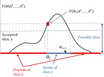
are shown in Alg. 5 and illustrated in Fig. 2.3.
There are many ways to extend this algorithm to a multidimensional setting. We
consider the simplest extension proposed by Neal [2003] where we use
hyperrectan-gles instead of intervals. A hyperrectangle region is constructed around Θi and the
edge in each dimension is expanded or shrunk depending on whether its endpoints
lie inside or outside the slice. One could alternatively consider coordinate-wise or
Figure 2.3: Illustration of the univariate slice sampling algorithm. In the first step, A slice yis generated by sampling from Uniform[0, P(Θi|A1, . . . , AT)]. Once a slice
Algorithm 5 Univariate Slice Sampling
Input: Starting point: Θ0, Initial width: w, Prior distribution: P(Θ), Samples:
X = [X1, . . . , XT].
Θ = Θ0
for i= 0 : (τ −1)do
y∼Uniform[0,P(Θi|A1, . . . , AT)]
z ∼Uniform[0,1]
L= Θi−z∗ w2
R =L+ w2
while y >P(L|A1, . . . , AT) do
L=L− w2
while y >P(R|A1, . . . , AT) do
R=R+ w2
ˆ
Θ∼Uniform[L, R]
if P( ˆΘ|A1, . . . , AT)< y then
while P( ˆΘ|A1, . . . , AT)< y do
if Θˆ >Θthen
R= ˆΘ
else
L= ˆΘ
ˆ
Θ∼Uniform[L, R] Θi+1 = ˆΘ
Chapter 3
Large-Scale Inference of Discrete
DPPs
An appealing aspect of a DPP defined on a discrete space, Ω ={x1,x2, . . . ,xN}is
its efficient sampling algorithm. Despite the probability distribution being defined
on the 2N of all possible subsets of Ω, the DPP sampler of Hough et al. [2006]
leads to an O(N3) algorithm (see Sec. 2.1.2). Imagine, however, machine learning
applications such as video summarization where each video might contain tens of
thousands of frames or possibly more. Suppose we are interested in selecting a
diverse subset from this set of frames by sampling from a discrete DPP. In this case,
when N is very large, an O(N3) algorithm can be prohibitively slow. Furthermore,
while storing a vector of N items might be feasible, storing anN×N matrix often
is not.
When the kernel matrix can be decomposed as L=B>B, where B is a D×N
matrix and D N, as presented in Sec. 2.1.5, Kulesza and Taskar [2010] offer
a solution by considering sampling from the dual representation. Recall that in
these cases sampling can be done in O(D3) time without ever constructingL. If
randomly projecting B into a lower-dimensional space. Gillenwater et al. [2012]
showed how such random projections yield an approximate model with bounded
variational error.
However, linear decomposition of the kernel matrix using low-dimensional (or
even finite-dimensional) features may not be possible. Even a simple Gaussian
ker-nel has an infinite-dimensional feature space, and for many applications, including
video summarization, the kernel can be even more complex and nonlinear.
Here we address these computational issues by approximating a DPP kernel
matrix L with a low rank matrix ˜L. There are many low-rank approximation
methods with results that are well documented both empirically and theoretically.
However, there are significant challenges in extending these results to the DPP.
Most existing theoretical results bound the Frobenius or spectral norm of the
kernel error matrix, but we show that these quantities are insufficient to give useful
bounds on distributional measures like variational distance. Instead, we derive
novel bounds for low-rank approximation that are specifically tailored to DPPs,
nontrivially characterizing the propagation of the approximation error through the
structure of the process.
One such approximation method that satisfies the hypothesis in our bounds is
the Nystr¨om method presented in Sec. 2.3.1. Our bounds are provably tight in
certain cases, and we demonstrate empirically that the bounds are informative for
a wide range of real and simulated data. These experiments also show that the
proposed method provides a close approximation for DPPs on large sets.
Another approximation method is the random Fourier features (RFF) presented
in Sec. 2.3.2. Here, however, the method does not satisfy our hypothesis making
theoretical analysis much more difficult. We will present an empirical comparison
useful in cases where there is low-correlation between the items.
Finally, we apply our techniques to select diverse and representative frames
from a series of motion capture recordings. Based on a user survey, we find that
the frames sampled from a Nystr¨om-approximated DPP form better summaries
than randomly chosen frames.
3.1
Low-Rank Approximated DPPs/
k
DPPs
While the dual representation of DPPs may not be available in many cases (such
as cases where L is generated by infinite-dimensional features), the dual DPP
sampling outlined in Sec. 2.1.5 can still be harnessed when one approximates L
with a low-rank matrix ˜L. Such an r-rank approximation to Lcombined with the
application of the the dual sampling reduces the complexity to O(r3+N r) time
and O(N r) space.
Most analysis of the error of low-rank approximations has been limited to
the Frobenius and spectral norms of the residual matrix L−L˜, such as the ones
presented in Secs. 2.3.1 and 2.3.2. While matrix norm bounds kL−L˜kF and
kL−L˜k2 are useful in quantifying the effectiveness of the low-rank approximation
methods in recovering the kernel matrix, it is not clear how these error bounds
propagate to quantifying the error in the DPP distributions. Specifically, since
the probability of sampling a specific subset A under a DPP is related to the
square of the volume spanned by the feature vectors of items in A (see Sec. 2.1).
Unfortunately, for many of these low-rank approximation methods, no volumetric
error bounds exist. The challenge here is to study how low-rank approximations
simultaneously affectsall possible minors of L.
In fact, a small error in the matrix norm can have a large effect on the minors
Example 1 Consider matrices L= diag(M, . . . , M, ) andL˜ = diag(M, . . . , M,0)
for some large M and small . Although kL−L˜kF = kL−L˜k2 =, for any A that
includes the final index, we have det(LA)−det( ˜LA) = Mk−1, where k=|A|.
It is conceivable that while errors on some subsets are large, most subsets are
well approximated. Unfortunately, this not generally true.
Definition 1 The variational distance between the DPP with kernel L and the
DPP with the low-rank approximated kernel L˜ is given by
kPL− PL˜k1 =
1 2
X
A∈2Ω
|PL(A)− PL˜(A)| . (3.1)
The variational distance is a natural global measure of approximation that ranges
from 0 to 1. Unfortunately, it is not difficult to construct a sequence of matrices
where the matrix norm of L−L˜ tends to zero but the variational distance does
not.
Example 2 Let L be a diagonal matrix with entries 1/N and L˜ be a diagonal
matrix with N/2 entries equal to 1/N and the rest equal to 0. Note that ||L−
˜
L||F = 1/
√
2N and ||L−L˜||2 = 1/N, which tend to zero as N → ∞. However,
the variational distance is bounded away from zero. To see this, note that the
normalizers are det(L+I) = (1 + 1/N)N and det( ˜L+I) = (1 + 1/N)N/2, which
tend toe and √e, respectively. Consider all subsets which have zero mass in the
approximation, S = {A : det( ˜LA) = 0}. Summing up the unnormalized mass
of sets in the complement of S, we have P
A /∈Sdet(LA) = det( ˜L+I) and thus
P
the sets in S to the variational distance:
kPL− PL˜k1 ≥
1 2
X
A∈S
det(LA)
det(L+I) −0
(3.2)
= det(L+I)−det( ˜L+I)
2 det(L+I) , (3.3)
which tends to e− √
e
2e ≈0.1967 as N → ∞.
One might still hope that pathological cases occur only for diagonal matrices,
or more generally for matrices that have high coherence [Candes and Romberg,
2007]. In fact, coherence has previously been used by Talwalkar and Rostamizadeh
[2010] to analyze the error of Nystr¨om approximations. Define the coherence
µ(L) = √Nmax
i,j |vij| , (3.4)
where each vi is a unit-norm eigenvector of L. A diagonal matrix achieves the
highest coherence of √N and a matrix with all entries equal to a constant has the
lowest coherence of 1. Suppose that f(N) is a sublinear but monotone increasing
function with limN→∞f(N) = ∞. We can construct a sequence of kernelsL with
µ(L) =pf(N) =o(√N) for which matrix norms of the low-rank approximation
error tend to zero, but the variational distance tends to a constant.
Example 3 Let L be a block diagonal matrix with f(N) constant blocks, each of
size N/f(N), where each non-zero entry is 1/N. Let L˜ be structured like L except
with half of the blocks set to zero. Note that µ2(L) =f(N) by construction and that
each block contributes a single eigenvalue of f(1N); the Frobenius and spectral norms
of L−L˜ thus tend to zero as N increases. The DPP normalizers are given by
det(L+I) = (1 + 1/f(N))f(N) →eand det( ˜L+I) = (1 + 1/f(N))f(N)/2 →√e. By
![Figure 2.1: A set of points in the plane drawn from a DPP (left), and the samenumber of points sampled independently using a Poisson point process (right).This figure is taken from Kulesza and Taskar [2012a].](https://thumb-us.123doks.com/thumbv2/123dok_us/9346514.1468895/23.595.168.463.109.261/figure-samenumber-independently-poisson-process-gure-kulesza-taskar.webp)