Short-term Scheduling of Non-Cascaded Hydro-thermal System with Transmission Losses using Accelerated Particle Swarm Optimization Algorithm

(1)

20

Short-term Scheduling of Non-Cascaded Hydro-thermal

System with Transmission Losses using Accelerated

Particle Swarm Optimization Algorithm

Hafiz Zaheer Hussain1_{, Aun Haider}1*_{, Muhammad Salman Fakhar}2_{, Jameel Ahmad}1_{, Muhammad Asim} Butt1_{, Khawar Siddique Khokhar} 1

1. Department of Electrical Engineering, School of Engineering, University of Management and Technology, (UMT), Sector C-2, Johar Town, Lahore 54770, Pakistan

2. Department of Electrical Engineering, University of Engineering and Technology, Lahore * Corresponding Author: Email: [email protected]

Abstract

This paper presents the implementation of accelerated particle swarm optimization (APSO) algorithm fora non-cascaded hydro-thermal scheduling and economic dispatch problem with hydel power transmission losses. APSO is a single step position updating variant of PSO and due to its single step updating of particles, it is very fast in converging towards global optimization solution of non-linear economic dispatch problems, as compared to the other variants of PSO. Convergence rates of this implementation are compared with approaches presented in literature for the same problem. Our solution outperforms other solutions despite additional constraint of transmission losses.

Key Words

: Economic Dispatch; Hydro-Thermal Scheduling; Accelerated Particle Swarm Optimization

(APSO); Power Optimization.

1 Introduction

Hydro-thermal power generation is the most commonly used way to meet the electricity demands. The economic dispatch of thermal generating units suggests that fuel cost of each generator should be minimized at run time whereas water discharge rate is required to be scheduled for efficient operation of hydel power generating units. There is no fuel cost associated with hydel power plant, so the overall objective is to reduce the cost of thermal units. This problem is known as hydro-thermal scheduling. If this problem is solved for the time duration of maximum of one week, then this is a special type of hydro-thermal scheduling, known as short-term hydro-thermal scheduling. This problem is non-linear in nature [1]. The hydro-thermal scheduling problem, both in its cascaded and non-cascaded forms, has been the subject of investigation for several decades. However, in constrained nonlinear and multimodal optimization problems, it is not easy to search for a near global optimal solution using deterministic methods. A review of linear, nonlinear, quadratic, Newton programming and interior point methods applied to solve the power flow problems were discussed in [2-3]. Several optimization techniques like fast evolutionary programming [4], honey bee mating [5], genetic algorithm [6], improved PSO [7], self-organizing hierarchical PSO [8], and artificial bee colony [9] have been implemented to solve cascaded short-term hydro-thermal scheduling

problems. Kennedy and Eberhart were the first to propose particle swarm optimization (PSO) [10-11]. However, several variants of PSO such as neighborhood topologies in fully informed and best of neighborhood particle swarms [12], population structure and particle swarm performance [13], the FIPSO [14] have been reported in the literature that help in making the convergence rate fast and help in approaching towards the global optimum solution. Several optimization algorithms have been published to solve non-cascaded short-term hydro-thermal scheduling problem without considering power loss described in [15-20].A survey of the applications of PSO algorithm in the optimization process of power system operations [21], optimization method applied to solve the short-term hydro-thermal scheduling problem since 1990 to 2008 [22], and performance of PSO and FIPSO with considered constant and linearly decreasing weight strategies on Michaelwicz function have been presented in [23].

PSO has performed the best on these problems, both in finding the good approximations to the global optimum solution and also in achieving those solutions in less number of iterations. A variant of PSO known as accelerated PSO (APSO) has been introduced in [24]. APSO performs very well in finding the global best solutions in fewer number of iterations even for highly multimodal and non-linear functions like Michaelwicz 2-D function. Recently APSO has been effectively used in several areas like optimal design of substation

(2)

21 grounding grid [25], optimum design of frame structures [26], a new dual channel speech enhancement [27], charging plug-in hybrid electric vehicles [28], support vector machine for business optimization and applications [29] and combination of chaos and APSO discussed in [30].

This paper presents the implementation of APSO algorithm with the consideration of non-cascaded hydel power scheduling and economic dispatch of thermal units. To the best of our knowledge, the APSO algorithm is implemented on short-term hydro-thermal scheduling problem for the first time and the algorithm gives very good global best solution and reaches the global best in less numbers of iterations. The results have been presented and the convergence behavior of our proposed APSO with existing literature has been compared outperforming other approaches as described in [17-20].

2. Hydro-Thermal Scheduling

Problem

The system model of hydro-thermal power balance is shown in Figure 1. In this model, thermal electric transmission losses are ignored due to short distance between thermal power generation and load. The total load demand needs to be met by hydel and thermal power generating units after subtracting transmission losses. There is no fuel cost associated with hydel power plant, so the overall objective is to reduce the cost of thermal units of short-term hydro-thermal scheduling problem [1] and find out the convergence behavior of APSO algorithm.

Figure 1: Hydro-thermal power generation system model

The hydro-thermal scheduling cost function and constrains are formulated as follows.

𝑀𝑖𝑛 𝐹 = ∑ 𝑛 𝐹(𝑃 , ) (1) Where, F is the cost of operation of the thermal unit during the jth _interval, _𝑃

, is the thermal power generated by thermal unit, for any time in jth

scheduling interval and n is the number of hours in the scheduling interval which comprises of twelve hours in our case. This is the objective function used to minimize the total cost Ft of the short-term

hydro-thermal scheduling problem. Subject to:

𝑄 = ∑ 𝑛 𝑄 (2)

𝑄 < 𝑄 < 𝑄 (3)

𝑀𝑃 + 𝑃 − 𝑃 − 𝑃 = 0 (4)

𝑃 , < 𝑃 , < 𝑃 , (5)

𝑃 , < 𝑃 , < 𝑃 , (6)

𝑉 < 𝑉 < 𝑉 (7) Where Pthermal is the thermal power, Vis the volume

of water, Phydel is the hydel power and Q is the water

discharge rate. In a reservoir, the volume of water Vj in the jth interval, is the function of the discharge

rate Qj, inflow rate Rjand spillage rate Sj in the jth

interval [1]. Reservoir volume at j+1 interval is:

𝑉 = 𝑉 + 𝑛 (𝑅 − 𝑄 − 𝑆 ) (8)

2.1. Problem of Interest

The problem of interest taken is the similar as tested in [1, 15-20]. All the experimental conditions are same as used in those references and the corresponding hydro-thermal system. Total thermal unit operational cost F, as a function of thermal power, can be modeled as a quadratic function as defined below:

𝐹 = 500 + 8(𝑃 ) +

0.0016(𝑃 ) (9)

Subject to:

150MW<(𝑃 )<1500MW Fuel Cost=1.15($/MBTU)

In hydel power system flow rate Q is major factor. So, total flow rate is expressed as a function of hydel power

For 150MW<(𝑃 )<1500MW

𝑄 = 330 + 4.97𝑃 (𝑎𝑐𝑟𝑒 𝑓𝑡 /ℎ𝑟) (10) For 150MW<(𝑃 )<1500MW0

(3)

22

𝑄 = 5300 + 12 𝑃 − 1000

+ 0.05 𝑃 − 1000 (11)

The distance between hydel plant and load is large, so the hydel electric transmission losses are modeled as:

𝑃 = 0.0008𝑃 𝑀𝑊 (12)

2.1.1. Discharge Rate Constraints

For the test model, the discharge rate should be within the range as follows:

For 0 ≤𝑃 ≤ 1000𝑀𝑊, discharge rate must be

300(𝑎𝑐𝑟𝑒 𝑓𝑡 /ℎ𝑟) ≤ 𝑄 ≤ 5300(𝑎𝑐𝑟𝑒 𝑓𝑡 /ℎ𝑟)

For 1000 ≤𝑃 ≤ 1100𝑀𝑊, discharge rate must be

5300(𝑎𝑐𝑟𝑒 𝑓𝑡 /ℎ𝑟) ≤ 𝑄 ≤ 7000(𝑎𝑐𝑟𝑒 𝑓𝑡 /ℎ𝑟)

2.1.2. Water Reservoir Constraints

Water reservoir constraints and characteristics are: 1. 100,000 acre-feet is the volume of water in

the reservoir at the start of scheduling. 2. 60,000 acre-feet is the volume of water in the

reservoir at the end of scheduling. 3. Volume constraints in acre-ft

60,000 (acre ft) ≤ V≤ 120,000 (acre ft) 4. Continuous Incoming flow into the reservoir

is 2000 acre-feet/hour throughout the scheduling period.

5. The continuity equation is

𝑉𝑜𝑙𝑢𝑚𝑒 = 𝑉𝑜𝑙𝑢𝑚𝑒 10. + 𝐼𝑛𝑓𝑙𝑜𝑤 −

𝐷𝑖𝑠𝑐ℎ𝑎𝑟𝑔𝑒 − 𝑆𝑝𝑖𝑙𝑙𝑎𝑔𝑒 𝑛 (13)

Spillage has been ignored in this problem formulation.

2.1.3. Schedule of Load Demand

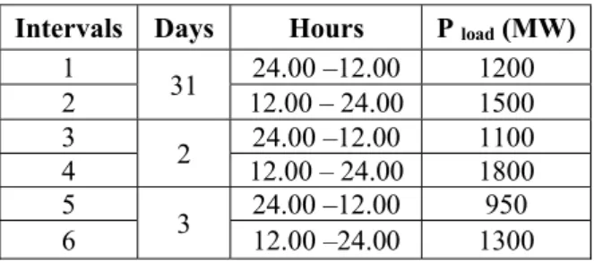
Table 1: Load demand in MW on different time intervals.

Intervals Days Hours P load (MW)

1 ₃₁ 24.00 –12.00 1200

2 12.00 – 24.00 1500

3

2 24.00 –12.00 1100

4 12.00 – 24.00 1800

5

3 24.00 –12.00 950

6 12.00 –24.00 1300

Load demand is scheduled as shown in Table 1.

3. Accelerated PSO

Accelerated PSO algorithm was developed by Yang [24] at the University of Cambridge in 2007 in order to accelerate the convergence behavior of the algorithm. As Compared to many PSO variants, APSO uses only two parameters, and the mechanism is simple to understand [28]. The amendment in the original PSO algorithm can be mathematically modeled as follows:

𝑣 = 𝑣 + 𝛼𝜀 𝑃_ − 𝑥 + 𝛽𝜀 𝑃 − 𝑥

(14) Where, α and β are the learning parameters or acceleration constants, 𝜀is a random variable, vi j is

ith velocity vector at jth_iteration,_𝑣 _{is the}_i_th

updated velocity vector at j+1 iteration, 𝑥 is the current position of the particle iat jth

iteration,𝑃_ is the global best and𝑃_ is the current best at jth_{iteration, equation (15) is the}

standard velocity equation of PSO algorithm. The new APSO form is derived when an inertia function

𝜃(𝑗) is used in a standard velocity equation of the PSO algorithm which is explained below:

𝑣 = 𝜃(𝑗) 𝑣 (15)

𝑣 = 𝜃(𝑗) 𝑣 + 𝛼𝜀 𝑝 _{_} − 𝑥 +

𝛽𝜀 (𝑝_{_} − 𝑥 ) (16) Where, 𝜃lies in between 0 to 1. Inertia function normally takes 𝜃 ≈ 0.5~0.9 as a constant. Inertia function is used to stabilize the motion of the particles by introducing the virtual mass. So, the algorithm will converge more rapidly as well as to stabilize the motion of the particles. The standard particles swarm optimization uses both local and global best of particle to evolve to the next position. The reason behind using the local best is to increase the variety in the quality solution; however, this diversity can be simulated using randomness. Local best can only be used when the problem is more complicated, multimodal and highly nonlinear [24]. As its name shows, accelerated PSO converges to the solution more quickly by using global best value only in the particle updating equation. So, the velocity vector is generated in the APSO using equation (16).

𝑣 = 𝑣 + 𝛼 𝜀 − + 𝛽 𝑝 _{_} − 𝑥 (17)

Where, 𝜀 is a random variable and its value lies between [0 -1]. The updated position formula is:

(4)

23 In order to further increase the convergence rate of

the APSO algorithm, put the value of the updated velocity vector 𝑣 in equation (17)

𝑥 = (1 − 𝛽)𝑥 + 𝑣 + 𝛽𝑝 _{_} + 𝜀 − 𝛼

(19) The initial velocity 𝑣 is zero at j=0, the new updated equation of the position vector becomes:

𝑥 = (1 − 𝛽)𝑥 + 𝛽𝑝 + 𝜀 − 𝛼 (20)

This is the simple single equation that uses only two parameters (α and β) in APSO algorithm. α and β are the learning parameters or acceleration constants, the typical values are: 𝛼 ≈

0.1~0.4 and𝛽 ≈ 0.1~0.7.𝛼 ≈ 0.2 and 𝛽 ≈

0.5can be taken as the initial values for the most uni-modal objective functions [24]. It is worth pointing out that the parameters α andβ should in general be related to scale the independent variables xi and the search domain. If, additional

improvement is required in APSO, to minimize the randomness as iterations continue, then a monotonically decreasing function for α can be used as given in eq.21.

𝛼 = 𝛼𝑒 (21) Or

𝛼 = 𝛼 𝛾 (0 < 𝛾 < 1) (22) Where, α0 is the initial value of the randomness

parameter its value isα0 ≈ 0.5~1 . jis the number of iteration and 𝛾 is a control parameter and its values are (0 < 𝛾 < 1) [24].

4. APSO Algorithm for Short-term

Hydro-Thermal Scheduling

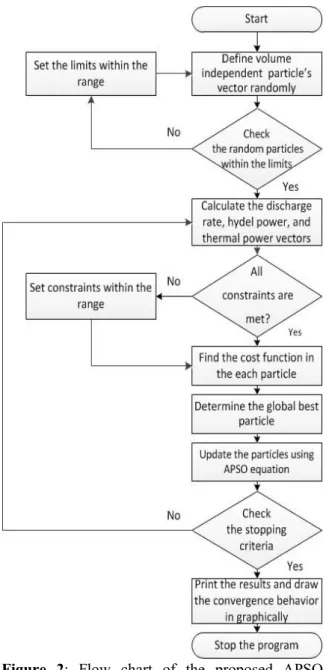
In the implementation of the Accelerated Particles Swarm Optimization algorithm on short-term hydro-thermal scheduling problem, there are four candidates’ variables; thermal power, volume of water, hydel power and water discharge rate for being the particles. In this implementation, the volume of water has been taken as an independent variable or particle and rest of three particles are taken as dependent variables. Figure 2 shows the flowchart of the APSO algorithm process. The steps to do the implementation are;

1. At the start, declare the population of particles, acceleration constants or learning parameters and the number of iterations. 2. The independent particle vectors, i.e. volume

vectors, are initialized randomly within its available reservoir constraint for each of the six scheduling intervals.

Figure 2: Flow chart of the proposed APSO algorithm.

3. Check whether the vectors of the volume particles are within the defined constraints or not, if not, then fix it within the limits. 4. Start the main iteration loop.

5. Generate the vector particles corresponding to discharge rate and check if the constraints are violated, then the discharge rate particles must be set within the defined constraints. 6. Produce the vector particles corresponding to

the hydel power and check if the constraints are violated. If there is violation, then the hydel power particles must be set within the defined limits.

7. After producing the hydel power vectors, generate the corresponding vectors of the thermal power, individual and optimal cost

(5)

24 and check if the constraints are within the defined limits. If so, then the particles must be set in the range.

8. For each iteration, calculate the desired fitness function using volume of water, discharge rate, hydel and thermal power vectors particles then compare these results with previous values using eq.9

9. The position of the particles location is updated by using eq.19

10. Repeat the procedure from step (V) until the giving criteria is met.

11. Get the desired results for economic scheduling.

12. Stop the algorithm.

5. Results

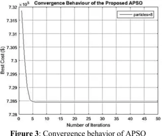
This section presents the implementations of the APSO algorithm on the formerly described short-term hydro-thermal scheduling problem with considered hydel transmission losses. Table 2 present the outstanding results of the selected problem when alpha=0.2, beta=0.5 and number of iteration=200 is considered. A statistical analysis

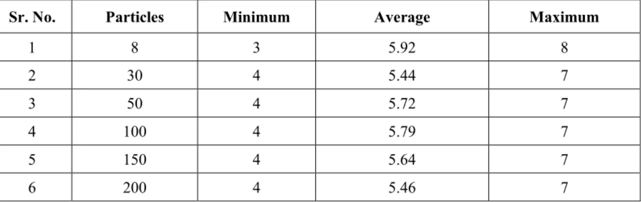
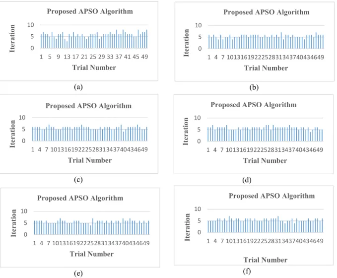
has also been presented to gauge the level of confirmation of the fact that APSO algorithm achieves a good approximate of the global best solution in very a few numbers of iterations. The algorithm is run on the short-term hydro-thermal scheduling problem with different numbers of particles in the APSO search swarm i.e. for 8, 30, 50, 100, 150, 200 particles separately and the convergence characteristics, for 50 number of iterations in each trial, of best cost in each of the iteration, are given in Figure 3 to 8 respectively. For each of the swarm size, 50 trials were made to have a statistical analysis of the convergence rate i.e. the numbers of iterations in which the solution is achieved, is presented in Figure 9 (a-f). Table 3 gives the average number of iterations, for each swarm size, in which the global minimum solution is achieved by the algorithm. It has been observed that, as the swarm size is increased, the APSO algorithm helps in achieving optimum solution presented in Table 4. This is because the search space is enhanced and each particle has more information as compared to when the particles of smaller swarm. However, on average the number of iterations in which the solution is achieved remains the same. The computation time of the APSO algorithm is relatively low.

Table 2: Power flow and cost optimization with APSO algorithm implementation (particles=200, alpha=0.2 and beta=0.5).

Interval 𝐏𝐝𝐞𝐦𝐚𝐧𝐝 (MW)

𝐏𝐭𝐡𝐞𝐫𝐦𝐚𝐥 (MW)

𝐏𝐥𝐨𝐬𝐬 (MW)

𝐏𝐡𝐲𝐝𝐞𝐥 (MW)

𝐐𝐝𝐢𝐬𝐜𝐡 𝐫𝐚𝐭𝐞 (acre ft /

hr)

𝐕𝐰𝐚𝐭𝐞𝐫 (acre ft)

Total Best Cost

($)

1 1200 842.1 10.8787 368.7603 2162.7 98047.137

727870

2 1500 964.3 25.1652 560.8606 3117.5 84637.412

3 1100 807 7.2116 300.2414 1822.2 86771.016

4 1800 1088.5 45.8952 757.4234 4094.4 61638.282

5 950 722.5 4.2985 231.7999 1482 67853.737

6 1300 849.8 17.4996 467.7018 2654.5 60000

Table 3: Statistical results of the maximum number of iterations using different swarm sizes.

Sr. No. Particles Minimum Average Maximum

1 8 3 5.92 8

2 30 4 5.44 7

3 50 4 5.72 7

4 100 4 5.79 7

5 150 4 5.64 7

(6)

25 Figure 3: Convergence behavior of APSO

algorithm using 8 particles swarm.

Figure 4: Convergence behavior of APSO algorithm using 30 particles swarm.

Figure 6: Convergence behavior of APSO algorithm using 100 particles.

(7)

26 (a)

(c)

(e)

(b)

(d)

(f)

Figure 9: Statistical representation of 50 independent trials at alpha=0.2 and beta=0.5 with (a) 8, (b) 30, (c) 50, (d) 100, (e) 150 (f) 200 particles.

Table 4: APSO results using different swarm sizes.

Sr. No. Power Losses Particles Number Parameters Cost ($)

Alpha Beta

1 Yes 8 0.2 0.5 728440

2 Yes 30 0.2 0.5 728130

3 Yes 50 0.2 0.5 727920

4 Yes 100 0.2 0.5 728090

5 Yes 150 0.2 0.5 727920

6 Yes 200 0.2 0.5 727870

6. Comparison of convergence

characteristics with previous

implementations

The convergence rate of APSO is very high as presented in Figs. (3-8). Convergence rates are compared with other implemented algorithms with

the help of graphs presented in Figures (10-13)) for the same problem. Our presented solution outperforms despite additional constraint of transmission losses. It can be observed that APSO converges to a good approximation of the global best solution very smoothly (without sticking for longer durations to local minima) and in a fewer numbers of iterations.

0 5 10

1 5 9 13 17 21 25 29 33 37 41 45 49

It

er

at

io

n

Trial Number Proposed APSO Algorithm

0 5 10

1 4 7 1013161922252831343740434649

It

er

at

io

n

0 5 10

1 4 7 1013161922252831343740434649

It

er

at

io

n

0 5 10

1 4 7 1013161922252831343740434649

It

er

at

io

n

0 5 10

1 4 7 1013161922252831343740434649

It

er

at

io

n

Trial Number

Proposed APSO Algorithm

0 5 10

1 4 7 1013161922252831343740434649

It

er

at

io

n

(8)

27 Figure 10: Convergence behavior of Improved

PSO by Padimini et al [17].

Figure 11: Convergence behavior of PSO [18].

Figure 12 (a): Convergence behavior of the meta-heuristic techniques [19].

Figure 12 (b): Convergence behavior of the meta-heuristic techniques [19].

Figure 13 (a): Convergence behavior of the FIPSO with l-best topology with 8 particles [20].

Figure 13 (b): Convergence behavior of the FIPSO with l-best topology with 50 particles [20].

(9)

28 Figure 13 (c): Convergence behavior of the FIPSO

with l-best topology with 100 particles [20].

Conclusion

Short-term hydro-thermal scheduling problem with hydel transmission power loss consideration has been solved using APSO algorithm to find the optimal scheduling cost with different swarm size and learning parameters. Because of the meta-heuristic nature of this algorithm, the statistical analysis is also presented. The program was run for 50 independent trials for several swarm sizes and the convergence characteristics for each were presented graphically. The results states that the proposed APSO algorithm has outperformed the existing various meta-heuristic and non-heuristic optimization techniques and given good final solutions. It has helped to achieve the results consistently and reaches the global minimum in a very few numbers of iterations. It used lesser number of particles to reach the best solution when compared to other forms of PSO algorithm. The computation time of the APSO algorithm is also relatively low. Transmission losses is the main reason of higher cost as compared to others, because in earlier works no transmission losses are used. Our presented solution outperforms previous work using meta-heuristic and non-heuristic optimization techniques despite additional constraint of transmission losses and has given relatively better results. The global minimum is achieved in a fewer number of iterations. If losses are increased the cost of generation will be increased and vice versa. Approximately there is 2.5% contribution of losses in the final best cost.

References

[1] Wood AJ, Wollenberg BF, Sheble GB. (2013). Power Generation, Operation and Control. IEEE & John Wiley.

[2] Momoh JA, Adapa R, El-Hawary ME. (1999). A review of selected optimal power flow literature to 1993. I. Nonlinear and quadratic programming approaches. IEEE Transactions on Power Systems, vol. 14, no. 1, pp. 96-104.

[3] Momoh JA, El-Hawary ME, Adapa R. (1999). A review of selected optimal power flow literature to 1993. II. Newton, linear programming and interior point methods. IEEE Transactions on Power System, 14(1), 105–11.

[4] Sinha N, Chakrabarti R, Chattopadhyay P. (2003). Fast evolutionary programming techniques for short-term hydro-thermal scheduling. Electric Power System Research, 66(2): 97–103.

[5] Tavakoli HB, Mozafari B, Soleymani S. (2012). Short-term hydro-thermal scheduling via honey bee mating optimization algorithm. Proceedings of the Asia pacific power and energy engineering conference (APPEEC), Shanghai, China, p. 1–5.

[6] Chen P, Chang H. (1996). Genetic aided scheduling of hydraulically coupled plants in hydro-thermal coordination. IEEE Transactions on Power Systems, 11 (2): 975– 981.

[7] Chang W. (2010). Optimal scheduling of hydro-thermal system based on improved particle swarm optimization. Proceedings of the Asia pacific power and energy engineering conference (APPEEC), 1–4. [8] Thakur S, Boonchay C, Ongsakul W. (2010).

Optimal hydro-thermal generation scheduling using self-organizing hierarchical PSO. Proceedings of the IEEE power and energy society general meeting, Minneapolis (USA), pp. 1–6.

[9] M. Basu. (2014). Artificial bee colony optimization for short-term hydro-thermal scheduling. Journal of the institute of engineers (India), Series B95 (4): 319-328. [10] Kennedy J, Eberhart R. (1995). Particle

swarm optimization. IEEE International Conference on Neural Networks Proceedings, 4, pp. 1942–1948.

[11] Eberhart R, Kennedy J. (1995). A new optimizer using particle swarm theory. Proceedings of the IEEE Sixth International Symposium on Micro Machine and Human Science, MHS95, pp. 39–43.

(10)

29 [12] Kennedy J, Mendes R. (2006).

Neighborhood topologies in fully informed and best of neighborhood particle swarms. IEEE Transactions System Man Cybernetics, Part C: Application and Review, 36(4), 515-519.

[13] J. Kennedy and R. Mendes. (2002). Population structure and particle swarm performance," Evolutionary Computation, 2002. CEC '02. Proceedings of the 2002 Congress on, Honolulu, HI, pp. 1671-1676. [14] R. Mendes, J. Kennedy and J. Neves. (2004).

The fully informed particle swarm: simpler, maybe better. IEEE Transactions on Evolutionary Computation, vol. 8, no. 3, pp. 204-210.

[15] Nallasivan C, Suman D, Henry J, Ravichandran S. (2006). A novel approach for short-term hydro-thermal scheduling using hybrid technique. Proceedings of the IEEE power India conference, New Delhi, India.

[16] Wong K, Wong Y. (1994). Short-term hydro-thermal scheduling part. I. Simulated annealing approach. IEEE Proceeding- Generation, Transmission and Distribution, 141(4), 497–501.

[17] Padmini S, Rajan C. (2011). Improved PSO for short-term hydro-thermal scheduling. Proceedings of the international conference on sustainable energy and intelligent systems, Chennai, India, pp. 332–334. [18] C. Samudi, G. P. Das, P. C. Ojha, T. S. Sreeni

and S. Cherian. (2008). Hydro thermal scheduling using particle swarm optimization. 2008 IEEE/PES Transmission and Distribution Conference and Exposition, Chicago, IL, pp. 1-5.

[19] Sinha N, Lai LL. (2006). Meta heuristic search algorithms for short-term hydro-thermal scheduling. Proceedings of the international conference on machine learning and cybernetics, Dalian (China).pp. 4050– 4056.

[20] Fakhar MS, Kashif SAR, Saqib MA, Hassan T. (2015). Non-cascaded short-term hydro-thermal scheduling using fully-informed particle swarm optimization. International Journal of Electrical Power and Energy Systems, 73, 983–990.

[21] Alrashidi MR, El-Hawary E. (2009). A survey of Particle Swarm Optimization Applications in Electric Power system.

Electric Power Component Systems, 13(4): 913–918.

[22] Farhat IA, El-Hawary ME. (2009). Optimization methods applied for solving the short-term hydro-thermal coordination problem. Electric Power Systems Research, 79(9):1308–1320.

[23] M. S. Fakhar1, S. A. R. Kashif, H.Z. Hussain, B. A. Ahmad. (2015). Implementation of PSO and FIPSO with consideration of constant and linearly decreasing weight strategies on Michaelwicz 3-D function. Sci. Int. (Lahore), 27(5), 4097-4100.

[24] Yang XS. (2010). Engineering optimization: an introduction with metaheuristic applications. John Wiley & Sons.

[25] El-Fergany, Attia. (2013). Accelerated Particle Swarm Optimization-based approach to the optimal design of substation grounding grid. Przeglad Elektrotechniczny. 89. 30-34.

[26] S. Talatahari, E. Khalili, and S. M. Alavizadeh. (2013). Accelerated Particle Swarm for Optimum Design of Frame Structures. Mathematical Problems in Engineering, vol. 2013, Article ID 649857, 6pages.

[27] Prajna K, Rao GSB, Reddy K, Maheswari RU. (2014). A New Dual Channel Speech Enhancement Approach Based on Accelerated Particle Swarm Optimization (APSO). I.J. Intelligent Systems and Applications, 04, 1-10.

[28] Rahman I, Vasant PM, Singh BSM, Al-Wadud (2016). A. On the performance of accelerated particle swarm optimization for charging plug-in hybrid electric vehicles. Alexandria Engineering Journal, 55(1), pp. 419–426.

[29] Yang, XS, Deb S, Fong S. (2011). Accelerated Particle Swarm Optimization and Support Vector Machine for Business Optimization and Applications. NDT2011, Springer, 136, pp. 53-66.

[30] Gandomi AH, Yun GJ, Yang XS, Talatahari S. (2013). Combination of chaos and accelerated particle swarm optimization. Communications in Nonlinear Science and Numerical Simulations, 18 (2), pp. 327–340.