Chemical and Biological Engineering Calculations using Python 3. Jeffrey J. Heys

Chemical and Biological

Engineering Calculations

using Python 3

Jeffrey J. Heys

This version is being made available at no cost. Please acknowledge access or use of the material by [email protected]. Tracking access and usage is professionally important to the author. Individuals that email the author will be alerted when revisions or corrections become available.

Formatting originally based on The Legrand Orange Book LA_{TEX template by Mathias Legrand.} Second printing, June 2015

Contents

1

1.1 Textbook and Course Format 9 1.2 Equation Identification and Categorization 10 1.2.1 Algebraic vs. Differential Equations . . . 10

1.2.2 Linear vs. Nonlinear Equations . . . 10

1.2.3 Ordinary vs. Partial Differential Equations . . . 11

1.2.4 Interpolation vs. Regression . . . 12

1.3 Problems 13 1.4 Additional Resources 14

2

2.1 Why Python? 15 2.1.1 Compiled vs. Interpreted Computer Languages . . . 16

2.1.2 A Note on Python Versions . . . 17

2.2 Getting Python 17 2.2.1 Installation of Python . . . 18

2.3 Python Variables and Operators 19 2.3.1 Containers . . . 20

2.4 External Libraries 22

2.5 Loops and Conditionals in Python 23

2.6 Functions 26

2.8.2 Array Operations . . . 30

2.9 Matplotlib Basics 31 2.10 Top 10 Common Python Error Messages and the Possible Cause 34 2.11 Problems 35 2.12 Additional Resources 38

3

3.1 Introduction 39 3.2 Symbolic Mathematics Packages 40 3.3 An Introduction to SymPy 40 3.4 Factoring and Expanding Functions 44 3.5 Derivatives and Integrals 46 3.6 Problems 48

4

4.1 Example Problem 52 4.2 A Direct Solution Method 54 4.2.1 Computational Cost . . . 58

4.3 Iterative Solution Methods 59 4.3.1 Vector Norms . . . 60

4.3.2 Jacobi Iteration . . . 60

4.3.3 Gauss-Seidel Iteration . . . 62

4.3.4 Convergence of Iterative Methods . . . 64

4.4 Problems 65

5

5.1 Motivation 69 5.2 Fitting Vapor Pressure Data 70 5.3 Linear Regression 71 5.3.1 Alternative derivation of the normal equations . . . 74

5.4 Nonlinear Regression 74 5.5 Problems 77

6

6.2 Bisection Method 83

6.3 Newton’s Method 86

6.4 Broyden’s Method 87

6.5 Multiple Nonlinear Equations 89

6.6 Problems 93

7

7.1 Introduction 97

7.2 Reading Data from a File 97

7.2.1 Parsing an Array . . . 100

7.3 Statistical Analysis 100

7.4 Advanced Linear Regression 103

7.5 Problems 106

8

8.1 Introduction 109

8.2 Numerical Differentiation 109

8.2.1 First Derivative Approximation . . . 110 8.2.2 Second Derivative Approximation . . . 112

8.3 Numerical Integration 113

8.3.1 Numerical Integration Using Scipy . . . 116

8.4 Problems 117

9

9.1 Introduction 119

9.2 Biochemical Reactors 119

9.3 Forward Euler 120

9.4 Modified Euler Method 123

9.5 Systems of Equations 124

9.5.1 Second-Order Initial Value Problems . . . 126

9.6 Stiff Differential Equations 126

9.7 Problems 129

10

10.1 Introduction 131

11

11.1 Finite Difference Method for Steady-State PDEs 141 11.1.1 Setup . . . 142

11.1.2 Matrix Assembly . . . 143

11.1.3 Solving and Plotting . . . 145

11.2 Including Convection 146 11.3 Finite Difference Method for transient PDEs 149 11.4 Problems 153

12

12.1 A Warning 155 12.2 Why FEM? 155 12.3 Laplace’s Equation 156 12.3.1 The Mesh . . . 156

12.3.2 Discretization . . . 156

12.3.3 Wait! Why are we doing this? . . . 157

12.3.4 FEniCS implementation . . . 157

12.4 Further Reading 158 Bibliography . . . 161

Textbook and Course Format

Equation Identification and Categorization

Algebraic vs. Differential Equations Linear vs. Nonlinear Equations

Ordinary vs. Partial Differential Equations Interpolation vs. Regression

Problems

Additional Resources

1. Problem Solving in Engineering

For most engineering problems, students find that the following sequence of steps is an effective problem solving approach to the vast majority of the problems they encounter:

Problem Statement System Diagram Model Equations Solution

Figure 1.1: Engineering problem solving process.

In most courses, students practice all the steps outlined in figure 1.1, but the focus is usually on the construction of the system diagram and developing the mathematical equations for every unique type of process that is the focus of a particular course. Only limited attention is usually given to solving the mathematical equations that arise in a particular course because the assumption is that the student should have learned how to do that in their mathematics courses or some other course. Many chemical or biological engineering curricula have a course that is focused on the use of computers to solve the many different types of equations that arise in a student’s engineering courses. The focus of this textbook is just that: using computers to solve the equation(s) that students typically encounter throughout the chemical and biological engineering curriculum.

The timing of a course on computational or numerical methods for solving engineering problems varies considerably from one curriculum to the next. One approach is to schedule the course near the end of the curriculum. As a upper level course, students are able to review most of the engineering principles and mathematics that they learned previously and develop a new set of tools (specifically, computational tools) for solving those same problems. Two disadvantages are associated with this approach. First, students do not have the computational tools when they first learn a new engineering principle, which limits the scope of problems they can solve to problems that can be largely solved without a computer (i.e., problems that can be solved with paper and pencil.) The second disadvantage is that the third- and fourth-years of many chemical or biological engineering curricula are already filled with other required courses and it is difficult to find time for yet another

course.

A second approach is to schedule the computational methods course early in the curriculum, before students have taken most of the engineering courses in which they learn to derive, construct, and identify the mathematical equations they need to solve and that sometime require a computational approach. There are also two problems with this approach. First, the students have typically not taken all the required mathematics courses, and, as a result, it is difficult to teach a computational approach to solving a differential equation when a student has not yet learned what a differential equation is or techniques for solving it. The second disadvantage is that the student has not taken courses on separations, kinetics, transport, etc. in which they learn to derive or identify the appropriate mathematical equation(s) for their particular problem. It is, of course, difficult to teach a computational approach to solving an equation when the importance or relevance of that equation is not known.

A third approach for addressing this dilemma is to simply not teach a stand-alone computational methods course and instead cover the relevant computational approaches as they are needed in each individual course. We will continue our listing of the ‘top two challenges’ and identify two potential difficulties with this approach. First, instead of learning and becoming comfortable with 2 or 3 computational tools (i.e., mathematical software packages), students under this format often need to learn 4 or 5 computational tools because every one of their instructors prefers a different tool, and the students never really become proficient with any single tool. The second difficult is that there are a few important concepts that play a role in many of the various computational methods, e.g., rounding error, logical operators, accuracy, etc., that may never be taught if there is not a single course focused on computational methods.

This textbook, and the course that it was originally written to support, are focused on the second approach – a course that appears in the first year or early in the second year of a chemical or biological engineering curriculum. The main reason for adopting this approach is simply the belief it is critical for students to understand both the potential power and flexibility of computational methods and also the important limitations of these methods before using them to solve problems in chemical and biological engineering. For a student to use a computational tool in a course and blindly trust that tool because they don’t understand the algorithms behind the tool is probably more destructive than never learning the tool at all. Further, to limit a student to only problems that can be solved with paper and pencil for most of their undergraduate education is similarly unacceptable. Addressing the limitations associated with teaching computational methods before most of the fundamental engineering and some mathematics courses is difficult. The basic strategy employed by this book is to teach students to recognize the type of mathematical equation they need to solve, and, once they know the type of equation, they can take advantage of the appropriate computational approach that was covered in the course associated with this book (or, more likely, refer back to this book for the appropriate algorithm for their particular equation).

There is a second, and possibly more important, reason for learning this material early in the engineering education process. It is related to the fact that one of the most difficult skills for many science, engineering and mathematics students to master is the ability to combine a number of small, simple pieces together into a more complex framework. In most science, engineering and mathematics courses in high school and early in college, students learn to find the right equation to solve the question they are asked to answer. Most problems can be completed inone or twosteps. Problems in later courses, on the other hand, can often requirefive to tenor more steps, and can require multiple pages of equations and mathematics to solve. This transition from small problems that only require a few lines to large problems that require a few pages can be very challenging for

1.1 Textbook and Course Format 9

many science, engineering, and mathematics students. I believe that programming in general, and numerical computations, in particular, can be a great way to develop the skills associated with solving larger problems. Programming requires one to combine a number of simple logical commands and variables together into a more complex framework. Programming develops the parts of our brains that allow us to synthesize a number of smaller pieces into a much larger whole. A good analogy is building something complex (e.g., the Death Star) with LEGO bricks. This process requires one to properly and carefully combine a number of simple pieces into a much larger structure. The entire process requires one to simultaneously think on both the large scale (‘What is my design objective?’) and the small scale (‘Will these two pieces stay connected? Are they compatible?’). This skill is necessary for both programming and engineering. It is a skill that almost everyone is capable of developing, but it takes practice — so, we might as well start early!

This textbook advocates that students develop the following skills: (1) recognize the type of mathematical equation that needs to be solved – algebraic or differential? linear or nonlinear? interpolation or regression? ordinary or partial differential equation?, and (2) select and implement the appropriate algorithm. If students are able to develop these two skills, they will be equipped with a set of tools that will serve them well in their later engineering courses. These tools can be used by a student to check their work, even when they are primarily using paper and pencil to solve a problem. It is not optimal that students learn how to approximately solve mathematical equations before they know why the equation is relevant, but every effort is made in this book to at least try and explain the relevance of equations when possible.

1.1 Textbook and Course Format

The course that motivated the creation of this textbook is one semester of approximately 15 weeks. It is the author’s belief that most of this material can be covered in that length of time. Each chapter in the textbook covers a different topic and was constructed so that the material in that chapter could be covered in approximately one week. There are, of course, some exceptions. For example, chapter 2 is one of the longest and may require two or even three weeks to cover. Conversely, chapter 3 is one of the shortest and can probably be covered in less than a week or omitted entirely. The large number of topics and short amount of time associated with a single semester, may encourage instructors using this book to consider a slightly different format than the traditional lecture format. For example, if two class times per week are available, an instructor may want to consider requiring students to read the book or watch an online lecture that presents the material to be covered before coming to the first class meeting time each week. The two class periods could then be used to cover example problems (the first class each week) and a ‘working class’ could be used for the second class meeting of the week. When students are trying to complete the homework, they often need support to overcome a difficult error message or unexpected and unphysical numerical answer from the computer, and allowing students to work on problems for one class time per week is often very beneficial.

Suggested homework problems are included at the end of each chapter. The homework problems are written so that the person answering the problem must respond to a request from a real or hypothetical organization such as a company or government agency. The author of this book typically assigns one or two problems per week and requires students to submit their solutions in the form of a memo to the organization that posed the problem. The memo typically is about one page of text, includes one to three figures, and the Python code is included in the appendix. Requiring students to practice technical writing is a benefit of using this approach, and many students are

motivated when the problems have more of a ‘real world’ flavor and are less abstract.

1.2 Equation Identification and Categorization

We identified two categories of skills that we wish to develop: (1) recognizing the type of mathemat-ical equation(s) and (2) selecting and implementing an appropriate computational method. The first skill will be covered in this first chapter and then the remainder of the book is for developing the second set of skills.

1.2.1 Algebraic vs. Differential Equations

The distinction between algebraic and differential equations is trivial – a differential equation is a relationship between the derivatives of a variable and some function. Differential equations described the rate of change of a variable; typically the rate of change with respect to space or time. Equations can have both independent and dependent variables. It is usually simplest to identify the dependent variables because their value depends upon the value of another variable. For example, in both v(t) =2π+t2and dv_dt =3+v·t,vis the dependent variable because its value depends on the value of tandtis the independent variable. There can be multiple independent variables, e.g., multiple spatial dimensions and time. In summary, differential equations have at least one derivative and algebraic equations do not. The presence of a derivative has a significant impact on the computational method used for solving the problem of interest.

1.2.2 Linear vs. Nonlinear Equations

A linear function, f(x)is one that satisfies both of the following properties: additivity: f(x+y) = f(x) +f(y)

homogeneity: f(c·x) =c f(x).

In practice, this means that the dependent variables cannot appear in polynomials of degree two or higher (i.e., f(x) =x2is nonlinear), in nonlinear arguments within the function (i.e.,f(x) =x+sin(x)

is nonlinear), or as products of each other (i.e., f(x,y) =x+xyis nonlinear).

For algebraic equations, it is typically straightforward to solve linear systems of equations, even very large systems consisting of millions of equations and millions of unknowns. Two different methods for solving linear systems of equations will be covered in chapter 4. Nonlinear algebraic equations can sometimes be solved exactly using techniques learned in algebra or using symbolic mathematics algorithms, especially when there is only a single equations. However, if we have more than one nonlinear equation or even a single, particularly complex nonlinear algebraic equation (or if we are simply feeling a little lazy) we may need to take advantage of a computational technique to try and find an approximate solution. Algorithms for solving nonlinear algebraic equations are described in chapter 6.

It is important to note that the distinction between linear and nonlinear equations can also be extended to differential equations and all of the same principles apply. For example, dc_dt =4c and d_dt22c =2 sin(πt) are linear while

dc dt =c

2 _{is nonlinear. In some cases, the nonlinearity will} not significantly increase the computational challenge, but, in other cases like the Navier-Stokes equations, the nonlinearity can significantly increase the difficulty in obtaining even an approximate solution.

1.2 Equation Identification and Categorization 11

1.2.3 Ordinary vs. Partial Differential Equations

An ordinary differential equation (ODE) has a single independent variable. For example, if a differential equation only has derivatives with respect to time,t, or a single spatial dimension,x, it is an ordinary differential equation. A differential equation with two or more independent variables is a partial differential equation (PDE). The following are examples of ordinary differential equations. Example 1.1

t·dc dt +

d2c

dt2 =sin(t) (linear, second-order ODE)

If you have not taken a differential equations course, this equation may look a little intimidating or confusing. To solve this equation, we need to find a functionc(t)where the first derivative of the function, multiplied byt, plus the second derivative of the function is equal to sin(t). If that sounds difficult, don’t worry, by the end of this textbook you will know how get an approximate solution, i.e., a numerical approximation of the functionc(t). It is also important to emphasize that multiplying the dependent variablecby the dependent variabletdid not make the equation nonlinear. A nonlinearity only arises if, for example,cis multiplied by itself.

Exercise 1.1 Even though you may not have taken a differential equations course, you might be

able to solve a simplified version of the previous example. Try to solve:

d2p

dt2 =sin(t)

Notice that we have eliminated the difficult term withtmultiplied by the first derivative. Let us start by integrating both sides of the equation with respect tot. Recalling that an integral is just an anti-derivative, so we get:

d p

dt +c1=−cos(t) +c2.

The two constants of integration can simply be combined into a single constant,c0, which can be placed on the right-hand side giving:

d p

dt =−cos(t) +c0.

Now, let us integrate both sides once more with respect tot:

p(t) +c3=−sin(t) +c0t+c4

which we can simplify once again by combining the two new constants of integration to a single constantc, to give:

p(t) =−sin(t) +c0t+c.

In order to fully determine our unknown function p(t), we need two additional conditions to solve for the value of our two remaining unknown constants,c0andc. Typically, this additional information would be initial conditions, i.e., the value ofp(0), i.e., the value ofpwhent=0, and the value ofd p_dt att=0.

It is always a good idea to check the solution to your problem by substitutingp(t)back into the original differential equation and checking to make sure that you get the desired right-hand

side.

Example 1.2 dx dt =x

2_{+3 cos(t) (nonlinear, first-order ODE) .}

Again, if you have not had a differential equations course, solving this equation requires finding a functionx(t)that has a derivative equal to(x(t))2plus 3 cos(t). Do not worry if that makes your head spin, we will also cover the solution of this class of problems.

Some examples of partial differential equations are included below. Example 1.3

∂T ∂t =α

∂2T

∂x2 (linear, second-order PDE),

This is an equation that describes unsteady, conductive heat transport in one spatial dimension. You could use this equation to describe, for example, the warming of the ground when the sun comes up in the morning, among many other examples. Solving this equation requires finding a function T(x,t)of both timetand spacexwhere the first derivative with respect to time is equal toα times

the second derivative with respect to space.

Example 1.4 m∂m

∂x + ∂m

∂y =0(nonlinear, first-order PDE).

By now it is probably obvious that the standard mathematical convention is to use∂for derivatives in a PDE while ODEs used. The order of the equation is determined by the order of the highest

derivative.

1.2.4 Interpolation vs. Regression

Within engineering, it is often necessary to obtain an equation, usually a polynomial equation, that ’fits’ a given set of data. If we want an equation that exactly matches the data, then we must interpolate the data so that we obtain a function (i.e., a polynomial) that has the same value as the data for a given value of the independent variable. In order to determine an interpolant, the number of adjustable parameters that we determine in the equation must equal the number of data points. For example, if we want to interpolate 3 data points, we must use an equation that has three adjustable parameters, such as a quadratic polynomial,ax2+bx+c.

1.3 Problems 13

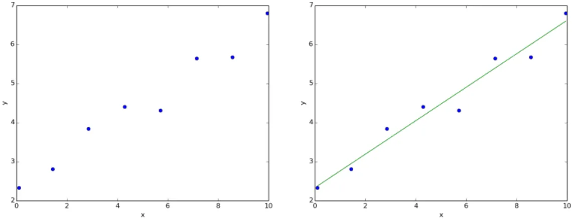
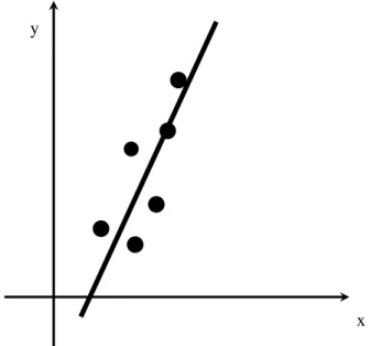
In practice, it is actually pretty rare that we want to exactly interpolate a given set of data because we hopefully have a large amount of data (and we don’t want to use a very high-order polynomial) and that data contains some amount of error. In most cases, we want to approximately fit our data with an equation of some form. In order to do this, we must first decide how we want to measure the ’goodness’ of a fit. Maybe we want to fit an equation so that the sum of the distances from the best fit equation to each and every point is minimized. Another option (the option that is almost always selected) is to minimize the sum of thesquareof the distance between every data point and the ’best’ fit approximation. This is the so called least-squares regression approach. The function that gives us the best fit based on our chosen criteria is called the regression function and the process of determining the regression function is called regression analysis. The most popular type of regression, linear regression (Figure 1.2) using least-squares, and nonlinear polynomial regression are both covered in chapter 5.

y

x

Figure 1.2: An example of linear regression for a given set of data.

1.3 Problems

Problem 1.1 Determine the type of differential equation:

(a) d_dt22x =−g(Newton’s first law) (b) ∂CA ∂t +v· ∂CA ∂z +kCA= ∂ ∂z D∂CA ∂z

Problem 1.2 If you want to determine the polynomial that interpolates 6 data points, what order

polynomial is required?

Problem 1.3 You are asked to use regression to determine the best linear polynomial fit for a given

set of data. A colleague encourages you to determine the best fit by minimizing the sum of the distance between each point and the line instead of minimizing the sum of the square of the distance, which is the standard practice. The colleague claims this will reduce the influence of a few outlying data points. Is the colleague correct?

1.4 Additional Resources

An understanding of how to solve differential equation problems is not required for understanding the material in this book. However, an ability to classify or recognize the type of equation that one is trying to solve is required. Most differential equation textbooks include a comprehensive set of definitions that enable the classification of mathematical equations. Two popular differential equation textbooks for engineers are:

• Differential Equations for Engineers and Scientists by Çengel and Palm [ÇP13] • Advanced Engineering Mathematics by Zill and Cullen [ZC06]

Why Python?

Compiled vs. Interpreted Computer Lan-guages

A Note on Python Versions

Getting Python

Installation of Python

Python Variables and Operators

Containers

External Libraries

Loops and Conditionals in Python Functions

Debugging or Fixing Errors Numpy Basics

Array and Vector Creation Array Operations

Matplotlib Basics

Top 10 Common Python Error Messages and the Possible Cause

Problems

Additional Resources

2. Programming with Python

The objective of this chapter is to motivate the use of the Python programming language for solving problems in chemical and biological engineering and then to present a few basic principles associated with programming in Python. It is important to emphasize that the goal is not to cover all aspects of programming in Python because that would require an entire book by itself. Instead, the goal is to present a few important principles and then slowly add additional Python programming knowledge throughout the remainder of the book.

2.1 Why Python?

When it comes to solving the many different mathematical problems that arise in chemical and biological engineering, many different software options exist for obtaining an exact or approximate solution. Some options, such as HYSYS and Aspen, are very user-friendly and they hide most of the details of the calculations from the user. While these software packages represent an important resource for engineers, our goal here is, in fact, to learn and understand the calculations that are happening in the background of these commercial packages. We will not discuss these high-level software packages here simply because we want to focus on and understand the actual computational details.

The next set of software options for solving engineering problems are mathematical software packages such as MATLAB, Mathematica, or MathCAD. These packages give the user more control over the calculations, but they also require more specialized knowledge than the process simulation software described previously. These mathematical software packages are probably the most popular options for a college-level course on chemical or biological engineering calculations. They have one major disadvantage, however, they can be quite expensive, especially if the various supporting libraries and add-on packages are also required. It is true that many institutions have a site license for these software packages, but the license may require students to be on the school’s network to use the software. It also means that the student is unlikely to have access to the software after they graduate.

your own computer code. Unfortunately, this option requires significant specialized knowledge — knowledge that is rarely retained beyond the course in which it is taught. Writing computer code can also be a very frustrating experience when subtle errors in the code are difficult to identify due to obscure error messages. The result is that students spend most of their time looking for errors in the computer code instead of learning about computations and algorithm development.

There is not a perfect solution to the dilemma of selecting an optimal computer environment for learning computational techniques for solving engineering problems. However, the Python programming language has many advantages that make it the platform of choice here. These advantages include:

1. It is freely available and runs on most major computer platforms including Windows, MacOS, and Linux.

2. It has a tremendous number of additional libraries that are also free and add computational mathematics capabilities. For example, the Numpy library provides Python with capabilities that are similar to those of MATLAB.

3. It is an interpreted language (defined below) and is easier and faster for developing new algorithms than compiled languages.

4. Many libraries of previously compiled algorithms can be imported into Python, which allows for very fast and efficient computations.

5. It is worth repeating – it is free!

2.1.1 Compiled vs. Interpreted Computer Languages

The first high-level programming languages that were developed, such as Fortran or C, were compiled languages. This meant that the programmer would type source code into the computer, this code was compiled into assembler code, and this was ultimately linked to produce a final executable file (see figure 2.1). The advantage of this approach is that the executable that was produced was relatively optimized and efficient for the platform on which it was built. Even today, most numerical software that requires significant computations, e.g., meteorological software, is written in a compiled language. The disadvantage of this approach is that significant expertise and training is required to write computer programs in a compiled language, identifying errors in the source code is often a very difficult and time consuming process, and the resulting program can only be run on the platform or operating system for which it is compiled.

These disadvantages associated with compiled programming languages can largely be addressed through the use of interpreted languages. Common interpreted programming languages include Java, Python, and JavaScript. Even MATLAB can be seen as an interpreted programming language. The source code for these languages is not compiled and linked to form a platform specific executable but is, instead, compiled to an intermediate language (or bytecode) that is run on a ‘virtual machine’. The virtual machine is a piece of software that interprets the bytecode and executes the instructions contained in the original source code. One obvious advantage of this approach is that the source code can be run on any computer that has the required virtual machine. Since Python and many associated libraries are available for all the major operating systems, you can execute Python source code almost anywhere. Interpreted languages also tend to be easier to program with because the syntax is more forgiving and the error messages are more informative (although you will still see cryptic error messages and frustrating syntax requirements in all computer languages). The disadvantage of interpreted languages is that they tend to execute instructions more slowly than compiled languages – often by a factor of 10 or more. If we need to multiply 1014numbers byπ, a factor of 10 can mean

2.2 Getting Python 17 Source Code Assembler Code Executable (platform specific) compiling linking Compiled languages: Interpreted languages: Source Code Intermediate representation

Virtual Machine (available on many platforms) compiling

(runtime)

Figure 2.1: The process of going from source code (i.e., a set of instructions) into a running computer program is different for compiled programming languages (top) versus interpreted programming languages (bottom).

the difference between a 1 hour computation and a 10 hour computation. Interpreted languages are getting faster all the time, however, and they are starting to close the gap between compiled and interpreted languages. One common strategy is ’Just-in-time’ (JIT) compilation. The basic idea here is that the virtual machine can actually compile important and frequently run source code all the way to a platform specific executable (just like a compiled language). Of course this ’on-the-fly’ compiling slows down the execution of the rest of the computer program, but, if a particular set of instructions is executed frequently, it may be more than worth the cost of JIT compilation.

2.1.2 A Note on Python Versions

In 2008, a new version of Python, Python 3.0, was released. This new version contained significant changes from the previous Python 2.x series. In particular, programs written for the Python 3.x series would normally not run on the Python 2.x series of virtual machines, and existing programs written for Python 2.x virtual machines would only occasionally run on Python 3.x series virtual machines. Because of these significant changes, the process of moving existing Python 2.x code so that it can execute on the newer Python 3.x series of virtual machines has progressed relatively slowly. As of 2015, most numerical python libraries are available for Python 2.7 or Python 3.x virtual machines. The examples in this textbook were written for a Python 3.x series virtual machine. It is inevitable that all Python computations will eventually transition to Python 3.x or later virtual machines. In the meantime, it is important to recognize the version of Python that use are using and select the appropriate virtual machine for the code that is being executed.

2.2 Getting Python

The process of learning numerical methods for chemical or biological engineering requires writing and executing computer programs. This book advocates the use of Python for writing and executing these computer programs so it is highly recommended that the reader have access to at least Python 2.7 plus the following libraries:

• Scipy (www.scipy.org) – scientific algorithm library that uses numpy

• Matplotlib (www.matplotlib.org) – provides the pyplot and pylab plotting libraries • SymPy (www.sympy.org) – symbolic mathematics library (optional, used primarily in Chapter

3)

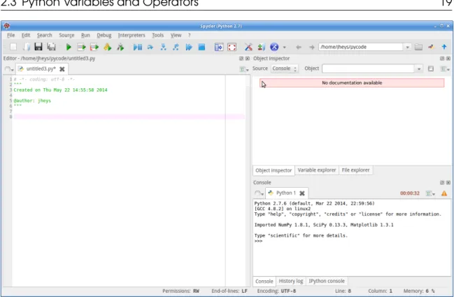
It is also recommended that an integrated development environment (IDE) be used to facilitate the writing of Python Source code. One particularly good IDE is called Spyder (code.google.com/ p/spyderlib). Figure 2.2 shows the basic layout of the Spyder IDE interface. The input window on the left side of the Spyder program window shows the Python source code that is currently being edited. The code in the source window can be executed or run by selecting ‘Run’ from the ‘Run’ menu or simply pressing F5 on most platforms. The upper right-hand screen usually shows documentation when it is available for different functions included with Python or imported libraries. The lower high-hand screen shows a Python console or Python prompt, ‘> > >’. Basically, the Python prompt is an actively running Python virtual machine and different Python commands can be tested at the prompt. The following exercise illustrates the power of and flexibility of the Python prompt.

Exercise 2.1 At the Python prompt, set the variable ‘a’ equal to the string ‘hello’, set the

variable ‘b’ equal to the string ‘world’ (note the space and the beginning), and then ask Python to ‘print(a+b)’. The exact sequence of instructions should give:

>>> a = ’ h e l l o ’ >>> b= ’ w o r l d ’ >>> p r i n t( a +b )

h e l l o w o r l d

Congratulations if you just executed your first Python program!

When writing a new Python program, it is often helpful to ‘try out’ a command or line of code at the Python prompt to observe the result. Having an active virtual machine for testing ideas helps to make Python an efficient language for writing new programs.

2.2.1 Installation of Python

For computers running Windows, three good options for installing Python include: • Anaconda Scientific Python (https://store.continuum.io/cshop/anaconda/) • pythonxy (code.google.com/p/pythonxy)

• winpython (winpython.sourceforge.net)

All of these packages include Python plus all the required libraries such as numpy and scipy plus they include the Spyder IDE. As of 2015, only Anaconda Scientific Python supported Python3. Presumably, the other options will eventually support Python3, but care should be taken when installing Python to select the desired Python version – 3.x or 2.x.

For computers running MacOS, it is easiest to install the Anaconda Scientific Python package (https://store.continuum.io/cshop/anaconda/).

For computers running a Debian-based version of Linux, the following command will install all required libraries:

sudo apt-get install python3-numpy python3-scipy python3-matplotlib ipython3

The FEniCS program, which is used in Chapter 12, is only available for Debian-based versions of Linux (i.e., Ubuntu or Mint Linux) or MacOS, and can be installed on Debian systems using

2.3 Python Variables and Operators 19

Figure 2.2: A screenshot of the Spyder IDE for Python programming including source code window on the left size, documentation window on the upper right side and Python console for rapid testing and executing the source code in the lower right side.

sudo apt-get install fenics

It should be noted that as of 2015, FEniCS requires Python 2.7, but it is expected to move to Python 3.x in the near future.

2.3 Python Variables and Operators

Programming frequently requires us to assign a variable to a specific piece of data (or something more complex). For example, typing:

a = " h e l l o "

into the console or a Python script file results in the variable ‘a’ beingassignedto character string ‘hello’. The wordassignedis emphasized here because it better reflects the role being played by the equal sign. Whenever Python code contains ‘=’, the object on the right is being assigned to the variable on the left.

In Python (and most other programming languages) we should see:

as

a←“hello”

The role of the assignment operator may seem obvious, but many programmers have struggled when the following code did not work:

>>> a =4 >>> a =b T r a c e b a c k ( m o s t r e c e n t c a l l l a s t ) : F i l e " < s t d i n > " , l i n e 1 , i n <module > N a m e E r r o r : name ’ b ’ i s n o t d e f i n e d >>>

The novice programmer may believe that the second line (‘a=b’) will result in ‘b’ being set to 4. This will not happen, and, instead, we get an error because the result of executing the code is that ‘a’ is assigned to something that is not defined (the variable ‘b’ has not been assigned). Notice that the end of the Python error message is telling us the problem.

Python usesstrong-typingfor variables, which means that every variable is a specific type, e.g., an integer, floating point number, character, etc. There is a built in function in Python calledtype() which will return the type for a given variable. In some cases it is possible to convert from one variable type into another variable type as is illustrated in the example below where a string (’str’) variable is converted into an integer (’int’).

>>> a = ’ 5 ’ >>> t y p e( a ) <t y p e ’ s t r ’ > >>> c =i n t( a ) >>> t y p e( c ) <t y p e ’ i n t ’ > 2.3.1 Containers

It is often useful in programming to collect multiple objects together into a single container and assign them to a variable. Python includes a number of different types of containers including tuples, lists, and dictionaries. The focus here is on numerical computations and the most useful type of container for these algorithms is a list container. In Python, a list has one or more objects (usually numbers for numerical computations) separated by commas and surrounded by square brackets. Lists may be heterogeneous – containing different objects types, but in practice, most lists only contain one type of variable. Lists should remind us of vectors. The construction of lists is illustrated below.

>>> v e c 1 = [ 2 , 3 , 5 ] >>> v e c 2 = [ 2 4 , 2 , 1 0 ] >>> v e c 1 . a p p e n d ( [ 8 , 2 ] )

2.3 Python Variables and Operators 21 >>> p r i n t( v e c 1 ) [ 2 , 3 , 5 , [ 8 , 2 ] ] >>> v e c 1 [ 3 ] = 87 >>> p r i n t( v e c 1 ) [ 2 , 3 , 5 , 8 7 ] >>> p r i n t( v e c 1 + v e c 2 ) [ 2 , 3 , 5 , 8 7 , 2 4 , 2 , 1 0 ] >>> p r i n t( v e c 1 + " w h a t ? " ) T r a c e b a c k ( m o s t r e c e n t c a l l l a s t ) : F i l e " < s t d i n > " , l i n e 1 , i n <module > T y p e E r r o r : c a n o n l y c o n c a t e n a t e l i s t (n o t " s t r " ) t o l i s t

Two vectors are defined at the console and assigned to the variable ‘vec1’ and ‘vec2’. To access an item in a list, use square brackets after the name of the variable, e.g., vec1[3] accesses the fourth item in the list. It is important to emphasize that in Python (and many other modern programming languages, the first item is a list has the index zero. To access the first item in vec1, use vec1[0]. Counting from zero can be awkward at first, but most experienced programmers appreciate the subtle advantages that will hopefully become apparent later.

After defining the vectors, a nested list is then appended onto the end of ‘vec1’ and then the nested list is replaced with 87 (programmers like to say that Python lists are mutable and can be changed). Lists of the same type can be concatenated as ‘vec1’ and ‘vec2’ are combined together. Lists of different types of objects cannot be concatenated as evidenced by the error message at the end.

Now that we know how to assign variables, we are in position to explore operators like ‘+’ and ‘*’, which allow us to effectively use Python like a calculator. The following example illustrates

some features of operators.

Example 2.1 The following can be typed into the Python console: >>> a =4

>>> b =2

>>> p r i n t( a−b ) 2

multiplication and division: >>> p r i n t( a∗b ) 8

>>> p r i n t( a / b ) 2 . 0

exponent and remainder: >>> p r i n t( a∗ ∗2 ) 16 >>> p r i n t( b%a ) 2 >>> p r i n t( a%b ) 0

2.4 External Libraries

Imagine that we want to calculate sin(1.2). If we try typing that into the Python console or a simple piece of source code, this is what we are likely to see:

>>> s i n ( 1 . 2 )

T r a c e b a c k ( m o s t r e c e n t c a l l l a s t ) : F i l e " < s t d i n > " , l i n e 1 , i n <module > N a m e E r r o r : name ’ s i n ’ i s n o t d e f i n e d

We get an error message because the sin()function is not a built-in function in Python. In order to use the sin()function, we need to import the ‘math’ library into Python. This can be accomplished two different ways and both are shown in the example below.

Example 2.2 To import a library, use theimportcommand

>>> i m p o r t math >>> math . s i n ( 1 . 2 ) 0 . 9 3 2 0 3 9 0 8 5 9 6 7 2 2 6 3

This is the preferred approach. The first command imports the entire math library , and any functions, methods, or data contained within that library can be accessed by typing: math.name or math.name() where name() is the name of a function in the library. A complete list of functions and values within the math library can be found atdocs.python.org/3/library/math.html.

The other approach to importing a library uses thefromcommand

>>> from math i m p o r t ∗ >>> s i n ( 1 . 2 )

0 . 9 3 2 0 3 9 0 8 5 9 6 7 2 2 6 3

This approach loads the entire math library into the global Python namespace, which can be thought of as a list of reserved words that are already defined. For example,import is a reserved word that is part of the global Python namespace and we should never useimportfor any other purpose. For example, do not try to use ‘import’ as a variable name. Whenever we load a library into this same global namespace, we greatly increase the number of global terms and invite the possibility of conflict. For example, if we tried to load two libraries that both contain the sin()function (both the math library and the Numpy library, which we use frequently both contain a sin()function), Python would give us an error. There are times when it is easier to use thefromnameimport∗option for loading libraries, but it is usually better to useimportname. If you tried to run >>> sin (1.2) at the console and were successful, this was a result of using an IDE that was smart enough to load the math library for you.

There are hundreds of libraries that have been written by others that increase the power of Python and save us from having to rewrite code that has already been written by others. In this book, we

2.5 Loops and Conditionals in Python 23

will use themath,numpy,scipyandpyplotlibraries extensively.

2.5 Loops and Conditionals in Python

As described previously, the equal sign does not actually compare two objects to see if they are equal. If we wish to compare two things for equality, we need to use == as illustrated:

>>> a =4 >>> b =4 >>> a ==b T r u e >>> a <b F a l s e

Beyond the equality comparator, the less than and greater than comparators are frequently helpful. In all cases, the comparator should return a boolean, True or False.

Example 2.3 While the focus in this textbook is on numerical programming, it can be interesting to try out some of the same principles on strings of characters. Consider the following:

>>> a = " h e l l o " >>> b= " w o r l d " >>> a ==b F a l s e >>> a <b T r u e >>> b< a F a l s e >>> p r i n t( a [ 1 : 4 ] ) e l l

Here the comparator compares two strings to determine which is first alphabetically. Comparators can be extremely helpful in constructing conditional statements. For example, if we want a block of code to only execute when a certain condition is true, we can use an if statement: >>> a =4 >>> i f a < 5 : . . . p r i n t( " s m a l l e r " ) . . . s m a l l e r

a =4 i f a < 3 :

p r i n t( " s m a l l e r " ) e l s e:

p r i n t( " l a r g e r " )

where the code will, of course, print ‘larger’ upon execution. From these two examples, we can make anINCREDIBLY IMPORTANT OBSERVATION (note that I wish that I could make the next sentence flash). In Python, blocks of code are designated using indentation. Every if statement has a condition followed by a colon. If the conditional is True the following block of text is executed, and the scope or length of the block is determined by the fact that all lines of code within the block MUST be indented EXACTLY the SAME amount. If the first line in the block is indented 4 spaces (and 4 spaces is the standard Python style), then every line must be indented 4 space. If you mess up and indent one line with only 3 spaces or a tab, error messages and chaos will follow. This same requirement extends to nested conditional statements, as shown.

Example 2.4 An example of nested conditional statements:

a =i n p u t( ’ E n t e r an i n t e g e r : ’ ) i f a > 3 : p r i n t( " a i s g r e a t e r t h a n 3 " ) p r i n t( " a d d i n g 1 " ) a += 1 # t h i s i s i d e n t i c a l t o a=a+1 i f a > 4 : p r i n t( " a i s g r e a t e r t h a n 4 " ) p r i n t( " s u b t r a c t i n g 1 " ) a −= 1 p r i n t( " a = " , a )

Upon execution with an input of ’4’, this code generates: a is greater than 3

adding 1

a is greater than 4 subtracting 1

a = 4

In the previous example we can also see an example of a ‘comment’ being include with the Python script. The comment, ‘# this is identical to a=a+1’ is included in the program to make it more readable and easier to understand. The use of frequent and descriptive comments is highly recommended. A good rule of thumb is that one comment should be included for every two lines of regular Python code. Another good rule of thumb is to use roughly an order of magnitude more comments in your own code compared to what you will find in this book! In Python, a comment is initiated by the ‘#’ character and all following characters are not interpreted or executed by the Python virtual machine – it is as if they do not exist. Optionally, multi-line comments can be initiated use three consecutive double quotes and ended using three consecutive double quotes. One final

2.5 Loops and Conditionals in Python 25

note, the comment character, ‘#’, can also be helpful for temporarily removing a line of code from execution.

One new Python function used in the previous example is theinput() function for getting input from the keyboard. The input from the keyboard is stored in the variable a in the example. It is alwaysa good programming practice to check the validity of input each and every time. In the above example, it would be good to check that a is between some minimum and maximum integers before using the variable any further.

Another situation where we have to be careful about indentation is loops. Loops allow us to repeatedly run a block of code for either a set number of iterations or until some condition is met. Theforloop is the most common type of loop and is illustrated below.

Example 2.5 Let us construct a loop that executes 5 times and has a counter that incrementally increases in value every time through the loop.

i m p o r t math

f o r i i n r a n g e( 5 ) : j = math . s i n ( i ) p r i n t( i , j ) p r i n t( " f i n i s h e d " )

Upon execution, the output from this code should be: 0 0 . 0 1 0 . 8 4 1 4 7 0 9 8 4 8 0 7 8 9 6 5 2 0 . 9 0 9 2 9 7 4 2 6 8 2 5 6 8 1 7 3 0 . 1 4 1 1 2 0 0 0 8 0 5 9 8 6 7 2 4 −0.7 56802 49530 79282 f i n i s h e d

Exercise 2.2 Therangefunction in Python supports the following arguments:

range( start , stop , step ). If only one input is given, it is treated as the stop value and the function returns the integers from 0 to stop−1. If two values are given, they are treated as start and stop values, and 3 values are treated as start, stop, and step size. Using this information, try to construct a loop that prints out the odd integers from 7 to 17, including 17.

We need to set start to 7, step should be set to 2 so that we only have odd integers, but how do we get the loop to include 17, but exclude 19?

The following will not work: f o r i i n r a n g e( 7 , 1 7 , 2 ) :

p r i n t( i ) p r i n t( " f i n i s h e d " )

This code will stop at 15. Instead, becauserangedoes not include the value of stop in the sequence, we need to set stop to 18 or 19. You may also want to try setting the value of start to 7.5 or some other non-integer. The result will not be good becauserangerequires all input

values to be integers.

2.6 Functions

We have already used a number of built-in functions and functions from external libraries, include the math. sin andrangefunctions. In many situations, it is very helpful to write our own functions. Advantages of writing functions include the fact that it becomes easier to reuse the code you have written previously, and functions help to break our programs up into manageable pieces, which makes programming easier. The keyworddefis used to define a function in Python. This keyword should be followed by the name of the function and variable names for any inputs. The set of instructions that make up the function appear in the block below the fist line. The construction of a function is illustrated through the following examples.

Example 2.6 We want to write a function that will print out the area of a triangle given the size of the base and the height.

d e f t r i a n g l e ( b a s e , h e i g h t ) : a r e a = 0 . 5∗b a s e∗h e i g h t p r i n t( a r e a )

t r i a n g l e ( 2 , 3 )

Upon execution, this code should print ‘3.0’ to the console output. Of course having a function that just prints something to the screen after a calculation is probably not that useful. Instead, we should try to construct a function that returns the results of the calculations whenever possible. This can be illustrated by rewriting the function in the above example so that it returns the area (and then prints it to the screen).

d e f t r i a n g l e ( b a s e , h e i g h t ) : a r e a = 0 . 5∗b a s e∗h e i g h t r e t u r n a r e a

s i z e = t r i a n g l e ( 2 , 3 ) p r i n t( s i z e )

Note the use of the keywordreturnat the end of the triangle function.

Exercise 2.3 Write a function that can be given the number of people at a table. Then, the

function calculates the arc length for a single slice of pizza if a single 16-inch diameter pizza is to be divided evenly among the people at the table and everyone receives just one slice.

i m p o r t math d e f a r c l e n g t h ( n u m P e o p l e ) : c i r c u m f e r e n c e = 16∗math . p i i f ( n u m P e o p l e < 1 ) : p r i n t( " E r r o r : m u s t h a v e a t l e a s t one p e r s o n " ) r e t u r n 0

2.7 Debugging or Fixing Errors 27 e l s e:

l e n g t h = c i r c u m f e r e n c e / n u m P e o p l e r e t u r n l e n g t h

p r i n t( a r c l e n g t h ( 6 ) )

The code above should return 8.3776, indicating that each of the 6 people in the test problem should receive a slice with an arc length of 8.4 inches. You may want to try modifying the code so that it calculates the arc length when everyone receives more than one slice, but they all still

receive the same number of slices.

As we will see later, it is often useful to combine related functions together into a single file with afilename.py extension. These functions can then be imported into other programs later on using importfilename and called using filename . function . This is a great way to recycle code we have already written.

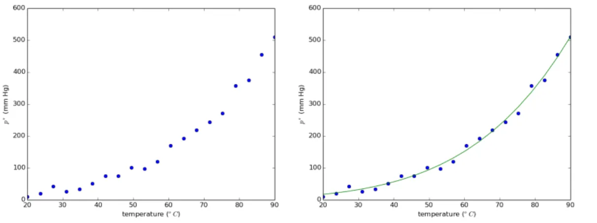
Exercise 2.4 The vapor pressure of a pure liquid, written p∗, is a strong function of temperature.

To calculate the vapor pressure at a given temperature,T, it is common to use Antoine’s equation:

log₁₀p∗=A− B T+C

whereA,B, andCare constants that can be looked up for different liquids. Write a function that hasA,B,C, andT (inoC) as inputs and returns the vapor pressure,p∗. Hint: 10log10x_=x.

Exercise 2.5 Write a function that hasA,B,C, and p∗(in mm Hg) as inputs and returns the

temperature,T.

2.7 Debugging or Fixing Errors

Probably the single greatest challenge that a novice programmer faces is correcting or fixing errors in their programs. The processes of correcting errors in computer code is commonly referred to as ‘debugging’. The origin of the term debugging is frequently attributed to Grace Hopper, an early computer pioneer who discoved a moth stuck in a computer relay that was causing errors. The topic of debugging is very broad and a large number of books have been written that are dedicated to the topic of debugging. Experienced computer programmers almost always use debugger software to help with the process of finding errors. Debugging software allows programs to be executed one or a few steps at a time while the value of various variables can be continuous tracked. This ability to run a program in ‘slow motion’ and with full variable exposure is very powerful. Debuggers for Python are included with most IDE’s include the Spyder IDE. While the use of debuggers is not described here, a few important strategies for finding and correcting errors are listed below.

1. The single most common mistake made by novice programmers is trying to write 10 or more new lines of code without testing the code. Experienced programmers try to test their programs after writing just a few (2 to 5) new lines of code. Ideally, programmers like to start with a similar, working code that can be modified a few steps at a time to reach the desired code. TEST OFTEN!!

2. Print out the value of variables whenever possible during the initial writing of the code to ensure that the code is behaving properly. These ‘print()’ statements are easy to remove later.

3. If a piece of code is not working, try to add a comment character, ‘#’, before as many lines as possible. Hopefully, this will allow the code to run. Then, remove the comment character one line at a time to find the line causing the problem.

4. Use the documentation available for the software libraries you are using to verify that the correct variable are being passed to functions in the library.

2.8 Numpy Basics

The numpy library adds powerful linear algebra data structures to Python. It allows us to construct and manipulate vectors and tensors very efficiently, and it is also widely used by other libraries that provide, for example, plotting and linear algebra solvers. The goal of this section is to provide a very brief introduction to a few important features of numpy. Throughout the rest of the book, additional features and options will be demonstrated. The online documentation and tutorials for numpy are also a very valuable source of information about the numpy library.

2.8.1 Array and Vector Creation

The are a number of different interfaces provided by numpy for constructing vectors and arrays. The simplest approach is to simply pass the numpy.array() method a Python list:

i m p o r t numpy

m y v e c t o r = numpy . a r r a y ( [ 5 , 3 , 7 ] , d t y p e =numpy . f l o a t 6 4 ) m y a r r a y = numpy . a r r a y ( [ [ 2 , 3 ] , [ 6 . 7 , 1 . 0 ] ] )

p r i n t( m y v e c t o r ) p r i n t( m y a r r a y )

If a single, 1-dimensional list is passed into the numpy.array() method, a 1-dimensional vector is created. It is optional to tell numpy the type of numbers that are stored in the array, integers, floats, or complex numbers. Using ‘float64’ causes every number in the array to be stored as a 64-bit floating point number. This is the default number type in numpy, so we will usually not set the ‘dtype’ option. If a nested list is passed into the numpy.array() method, a 2-dimensional tensor is created.

This approach to array construction works great for very small arrays where we already know the values. In practice, however, we will usually construct an array of zeros of the size we want, and then use loops to insert the desired values into the array. This approach is illustrated in the example below.

Example 2.7 Array construction by first initializing an array to zero and then using a loop.

i m p o r t numpy

s i z e = 3

m y a r r a y = numpy . z e r o s ( [ s i z e , s i z e ] )

f o r i i n r a n g e( s i z e ) : f o r j i n r a n g e( s i z e ) :

2.8 Numpy Basics 29

m y a r r a y [ i , j ] = 1 . 0 / ( i∗j + 1 . 0 )

p r i n t( m y a r r a y )

The program constructs a square, 2-dimensional array to whatever size is specified by the size variable. The zeros within the array are then replaced by the values calculated inside the nested loop. This approach to first allocating space for an array and then overwriting the initial values is typically more computationally efficient than first constructing an empty array and then appending values. We need to make a very important observation from the previous example: in Python, lists, vectors, and arrays are indexed starting with zero! In other words, if we have a vector that contains 5 numbers (i.e., it has length 5), those numbers are accessed with the indices 0, 1, 2, 3, and 4. Notice how if we loop from 0 to a number less than the size of the vector (in this case we loop from 0 to 4), we loop through all the indices without including 5. This important observation is important, and forgetting how vectors are indexed leads to many troublesome bugs in the code.

The final method that is sometimes helpful for array construction is to build an array where the values increase incrementally. For example, we might wish to construct and array of length 10 that contains the integers from 1 to 10. One nice feature of such a vector, is that it also allows us to demonstrate how to access a subsection of the vector.

Example 2.8 A sequential array and slicing:

i m p o r t numpy

m y a r r a y = numpy . a r a n g e ( 1 , 1 1 ) p r i n t( m y a r r a y )

m y a r r a y [ 3 : 6 ] = numpy . a r r a y ( [ 3 0 0 , 4 0 0 , 5 0 0 ] ) p r i n t( m y a r r a y )

The code in this example begins by constructing a vector from 1 to 11, but then, we replace 3 of the values within the vector with much larger values. Notice how we replace the values stored at indices 3,4, and 5 because the slicing command – 3:6 – does not include the last index (6) in the slice. Also recall the first entry in the vector (in this case ‘1’) is at index zero. So index 3 initially contains the value 4, which is replaced with 300. Then, the value at index 4, which is initially 5, is replaced with 400. The result of running the example code should be:

[ 1 2 3 4 5 6 7 8 9 1 0 ]

[ 1 2 3 300 400 500 7 8 9 1 0 ]

Example 2.9 The Fibonacci sequence is an important mathematical series that is frequently found in nature (e.g., the arrangement of sunflower seeds). The first two values in the sequence are defined as 0 and 1. Additional terms in the sequence are calculated by summing the previous two terms in the sequence. The function below stores the Fibonacci sequence in a numpy array.

s e q L e n g t h = 10 s e q = numpy . z e r o s ( s e q L e n g t h , d t y p e =numpy . i n t 3 2 ) s e q [ 0 ] = 0 s e q [ 1 ] = 1 f o r i i n r a n g e( 2 , s e q L e n g t h ) : s e q [ i ] = s e q [ i−1]+ s e q [ i−2] p r i n t( " F i n a l s e q u e n c e : " , s e q ) 2.8.2 Array Operations

To review, we have discussed the construction of numpy vectors and arrays, and we have discussed how to access the various entries within the vectors and arrays. Before closing out this very brief introduction to numpy, let us explore a few different operations that can be performed on matrices and vectors with the following example.

Example 2.10 Try running the code below:

i m p o r t numpy m y a r r a y = numpy . a r a n g e ( 5 ) p r i n t( m y a r r a y ) p r i n t( m y a r r a y . s h a p e ) m y a r r a y = m y a r r a y∗4 p r i n t( m y a r r a y ) y o u r a r r a y = numpy . o n e s ( 5 ) t h e i r a r r a y = m y a r r a y − 3∗y o u r a r r a y p r i n t( t h e i r a r r a y ) p r i n t( numpy . d o t ( m y a r r a y , t h e i r a r r a y ) ) i t s a r r a y = numpy . o u t e r ( m y a r r a y , t h e i r a r r a y ) p r i n t( i t s a r r a y ) p r i n t( i t s a r r a y . s h a p e )

This code segment begins by building a sequential vector of length 5. The ‘shape’ property of that vector should return ‘(5,)’, which tells us that the array has 5 rows and no additional columns. This initial vector is then multiplied by 4 and a second and third array are built. The third array, called ‘theirarray’ is actually built by taking the first array, ‘myarray’, and subtracting an array of 3’s from it. Please note that adding or subtracting one array from another requires that the arrays have the same size and shape – that is why it is often a good idea to print the value of size and shape to the screen so that you can confirm the sizes are the same. The example ends by taking a dot product of two vectors (again, they must have the same size) and an outer product. This example barely scratched the surface of what is possible with numpy. For example, we

2.9 Matplotlib Basics 31

have not yet covered matrix inversion or eigenvalue calculations, but many of these topics will be discussed in later chapters.

2.9 Matplotlib Basics

Matplotlib is one of many libraries that adds plotting capabilities to Python. It is a particular good choice here because it is well integrated with numpy and it provides relatively high quality output. To use Matplotlib within our Python scripts, we will import the either pylab library, which gives an interface similar to MATLAB’s plotting functionality, or the pyplot library. Pylab and pyplot provide the same functionality, but pylab is slightly easier to use from the Python prompt. Let us begin with a simple example.

Example 2.11 The following script builds a vector with 100 entries that span from 0 to 10.0 using numpy’s linspace() function. Then, pylab is used to generate a scatter plot wherexis from 0 to 10 andyis cos(x). i m p o r t numpy i m p o r t p y l a b x=numpy . l i n s p a c e ( 0 , 1 0 , num = 1 0 0 ) y = numpy . c o s ( x ) p y l a b . p l o t ( x , y ) p y l a b . show ( )

The resulting figure is shown on the left of Figure 2.3. The final line of example code (pylab . show()) is required because it causes the figure to persist on the screen and become in-teractive. If this line is omitted, the figures is either never plotted to the screen or is plotted for a fraction of a second before it disappears. Think of the pylab . show() function as causing the program to pause and wait for the user to decided what they want to do with the plot. The pylab . show() function is not required on all operating systems.

If the function call to pylab . plot (x,y) is replaced with pylab . plot (x,y, ’bo’), the plot is con-structed with blue circles instead of a solid line, as shown in the right half of figure 2.3.

It is also possible to place multiple curves on the same plot and include axis labels and figure titles as illustrated in the following example.

Example 2.12 This example shows the contour plot of a function with two independent vari-ables.

i m p o r t m a t p l o t l i b . p y p l o t a s p l t i m p o r t numpy a s np

x = np . l i n s p a c e ( 0 , 2 , 2 0 0 )

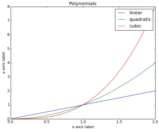
Figure 2.3: A figure of a cos()-wave generated using pylab with a solid line (left) and blue circles (right). p l t . p l o t ( x , x∗ ∗2 , l a b e l = ’ q u a d r a t i c ’ ) p l t . p l o t ( x , x∗ ∗3 , l a b e l = ’ c u b i c ’ ) p l t . x l a b e l ( ’ x−a x i s l a b e l ’ ) p l t . y l a b e l ( ’ y−a x i s l a b e l ’ ) p l t . t i t l e ( " P o l y n o m i a l s " ) p l t . l e g e n d ( ) p l t . show ( )

This example illustrates how every call to functions in the matplotlib library are applied to the current, active figure. This behavior is similar to Matlabe. Notice that axis labels are added to the figure using the plt . xlabel () and plt . ylabel () function calls with the desired string of text being passed into the function. A title is added to the figure using plt . title () function call, but, in common engineering practice, titles are not included for figures. In the future, we will use plt . figure () in the matplotlib library to generate additional figures and avoid having everything on the same figure. The result of running the example code is shown in figure 2.4.

Before ending this section, the power of Matplotlib is illustrated through a slightly more complex example.

Example 2.13 This example shows the contour plot of a function with two independent vari-ables.

i m p o r t p y l a b i m p o r t numpy

2.9 Matplotlib Basics 33

Figure 2.4: A plot showing a linear, quadratic, and cubic polynomial all on the same plot with a legend identifying each curve.

r e t u r n (1−x / 2 + x∗∗2+ y∗ ∗3 )∗numpy . exp (−x∗∗2−y∗ ∗2 )

n = 256 x = numpy . l i n s p a c e (−2 , 4 , n ) y = numpy . l i n s p a c e (−2 , 4 , n ) X , Y = numpy . m e s h g r i d ( x , y ) C = p y l a b . c o n t o u r ( X , Y , f ( X , Y ) , 8 ) p y l a b . c l a b e l ( C , i n l i n e = 1 ) p y l a b . c o l o r b a r ( C , o r i e n t a t i o n = ’ v e r t i c a l ’ ) p y l a b . show ( )

The function that is plotted is defined by the function f(x,y). The independent variables, x∈(−2,4)andy∈(−2,4), are stored in vectors created using numpy’s linspace() function. The numpy meshgrid function extends the 1-dimensional vectors over a 2 dimensional array. The contour plot consists of 8 contour lines, which are labeled, and a colorbar is added to the right of the plot. Colorbars are largely unnecessary and unattractive for this style of contour plot, but one is included here to illustrate the simplicity with which it can be added. The resulting figure is shown below (figure 2.5).

Figure 2.5: A contour plot of a function, f(x,y) = (1−x/2+x2+y3)exp(−x2_−y2_{)forx∈(−2,4)} andy∈(−2,4)

Matplotlib is a comprehensive plotting library, large enough that an entire book has been written to document all of the many different style of figures and options. For more information about the library as well as documentation describing the interfaces into the library, please see the tutorials posted on the library website:matplotlib.org.

2.10 Top 10 Common Python Error Messages and the Possible Cause

We end this chapter with a list of the 10 most commonly encountered error messages and some common causes for those messages.

1. TypeError - this error is caused by trying to use a variable of one type in a situation that requires a different type. For example, trying to combine an ‘int’ and a ‘str’. The TypeError message is usually followed by the actual variable type followed by the required variable type. 2. IndexError - this error is caused by trying to access part of a list or array that is beyond the

existing range. A frequent cause is forgetting that a list or array is indexed starting with zero. If an array (e.g., myarray) has 5 entries, then the 5th and final entry is accessed using an index of 4 (e.g., myarray[4]). In diagnosing the problem, it is often good to print the array to the screen to determine the current length.

2.11 Problems 35

The most common cause is forgetting a colon (‘:’) at the end of a line that requires one (e.g., lines starting with ‘if’, ‘while’, ’for’, etc.)

4. SyntaxError: EOL while scanning string literal - this is a special syntax error that is usually caused by forgetting a quotation mark or using a mixture of single ‘ and double “ quotation marks.

5. NameError - happens when you try to use a variable that has not been defined. This frequently occurs when we forget to initialize a variable to a value.

6. ZeroDivisionError - probably the easiest error message to understand, but it can be difficult to solve. It is always a good idea to print the values of variables to the screen to better understand when/how a variable is being set to zero instead of a non-zero value.

7. IndentationError - caused by inconsistent indentation in a block of code that should have been uniformly indented. Visual inspection can often reveal the problem unless the problem is caused by a mixture of ‘spaces’ and ‘tabs’. The solution is to not use ‘tabs’ or use an editor that converts ‘tabs’ into ‘spaces’.

8. AttributeError - happens when we try to call a function that does not exist (or we misspell a function that does exist) in a library (e.g., math.sine() instead of math.sin()).

9. KeyError - only occurs with dictionaries when we use a key that does not exist.

10. SyntaxError: invalid syntax - can happen if we try to use one of the reserved Python keywords as a variable. The Python 3 keywords are: and, as, assert, break, class, continue, def, del, elif, else, except, False, finally, for, from, global, if, import, in, is, lambda, None, nonlocal, not, or, pass, raise, return, True, try, while, with, yield. Many Chemical and Biological Engineers have struggled to fix this error when they tried to use ‘yield’ as a variable name.

2.11 Problems

Problem 2.1 Write a function called FtoC(T) that receives a temperature in Fahrenheit as the input

and returns the temperature in Celsius as the return value. Write a second function called CtoF(T) does the opposite – receives a temperature in Celsius as the input and returns the temperature in Fahrenheit. Demonstrate one of the functions by inputting the current temperature at the location of your birth using the standard temperature measurement unit at that location, and print out the temperature in the other system of units. For example, I was born in Bozeman, Montana, USA, so my input would be the current temperature in Fahrenheit, and I would print out the temperature in Celsius.

Problem 2.2 The LEGO Movie has what is quite possibly the most annoying theme song ever,

“Everything Is Awesome.” The lyrics for the chorus are reproduced below. Write a script that stores each line of the chorus as a separate string in a list. Then, input from the user a number corresponding to the number of lines that they would like printed to the screen. Check the number to determine that it is valid before printing the lines to the screen.

Everything is awesome

Everything is cool when you’re part of a team Everything is awesome when we’re living our dream

Everything is better when we stick together

Side by side, you and I gonna win forever, let’s party forever We’re the same, I’m like you, you’re like me, we’re all working in harmony