Lecture 12
Limit theorems. Basic inequalities. Central limit theorem.
Characteristic function.
Plan of the lecture:
1. Some useful inequalities
2. The Weak Law of Large Numbers (WLLN) 3. The Central Limit Theorem
4. The Strong Law of Large Numbers (SLLN) 5. Transforms
1 Some useful inequalities
In this lecture, we derive some important inequalities. These inequalities use the mean, and possibly the variance, of a random variable to draw conclusions on the probabilities of certain events. They are primarily useful in situations where the mean and variance of a random variable are easily computable, but the distribution of is either unavailable or hard to calculate.
We first present the Markov inequality. Loosely speaking it asserts that if a nonnegative random variable has a small mean, then the probability that it takes a large value must also be small.
Markov Inequality
If a random variable can only take nonnegative values, then
, for all .
To justify the Markov inequality, let us fix a positive number and consider the random variable defined by
It is seen that the relation
always holds and therefore,
.
On the other hand,
,
.
Example 1. Let be uniformly distributed on the interval [0, 4] and note that . Then, the Markov inequality asserts that
, , .
By comparing with the exact probabilities
, , ,
we see that the bounds provided by the Markov inequality can be quite loose.
We continue with the Chebyshev inequality. Loosely speaking, it asserts that if the variance of a random variable is small, then the probability that it takes a value far from its mean is also small. Note that the Chebyshev inequality does not require the random variable to be nonnegative.
Chebyshev Inequality
If is a random variable with mean and variance , then
, for all .
To justify the Chebyshev inequality, we consider the nonnegative random variable
and apply the Markov inequality with . We obtain
.
The derivation is completed by observing that the event is identical to the event and
An alternative form of the Chebyshev inequality is obtained by letting , where is positive, which yields
.
Thus, the probability that a random variable takes a value more than standard deviations away from its mean is at most .
The Chebyshev inequality is generally more powerful than the Markov inequality (the bounds that it provides are more accurate), because it also makes use of information on the variance of . Still, the mean and the variance of a random variable are only a rough summary of the properties of its distribution, and we cannot expect the bounds to be close approximations of the exact probabilities.
Example 2. As in Example 1, let be uniformly distributed on . Let us use the Chebyshev inequality to bound the probability that . We have , and
which is not particularly informative.
For another example, let be exponentially distributed with parameter , so that
. For , using Chebyshev’s inequality, we obtain
.
This is again conservative compared to the exact answer .
2 The Weak Law of Large Numbers (WLLN)
The weak law of large numbers asserts that the sample mean of a large number of independent identically distributed random variables is very close to the true mean, with high probability.
.
We have
,
and, using independence,
.
We apply Chebyshev’s inequality and obtain
, for any .
We observe that for any fixed , the right-hand side of this inequality goes to zero as increases. As a consequence, we obtain the weak law of large numbers, which is stated below. It turns out that this law remains true even if the have infinite variance, but a much more elaborate argument is needed, which we omit. The only assumption needed is that is well-defined and finite.
The Weak Law of Large Numbers (WLLN)
Let be independent identically distributed random variables with mean . For every , we have
, as .
The WLLN states that for large , the “bulk” of the distribution of is concentrated near . That is, if we consider a positive length interval around , then there is high probability that will fall in that interval; as , this probability converges to . Of course, if is very small, we may have to wait longer (i.e., need a larger value of ) before we can assert that is highly likely to fall in that interval.
According to the weak law of large numbers, the distribution of the sample mean is increasingly concentrated in the near vicinity of the true mean . In particular, its variance tends to zero. On the other hand, the variance of the sum increases to infinity, and the distribution of cannot be said to converge to anything meaningful. An intermediate view is obtained by considering the deviation of from its mean , and scaling it by a factor proportional to . What is special about this particular scaling is that it keeps the variance at a constant level. The central limit theorem asserts that the distribution of this scaled random variable approaches a normal distribution.
More specifically, let be a sequence of independent identically distributed random variables with mean and variance . We define
.
An easy calculation yields
,
and
.
The Central Limit Theorem
Let be a sequence of independent identically distributed random variables with common mean and variance , and define
.
Then, the CDF of converges to the standard normal CDF
in the sense that
, for every .
The central limit theorem is surprisingly general. Besides independence, and the implicit assumption that the mean and variance are well-defined and finite, it places no other requirement on the distribution of the , which could be discrete, continuous, or mixed random variables. It is of tremendous importance for several reasons, both conceptual, as well as practical. On the conceptual side, it indicates that the sum of a large number of independent random variables is approximately normal. As such, it applies to many situations in which a random effect is the sum of a large number of small but independent random factors. Noise in many natural or engineered systems has this property. In a wide array of contexts, it has been found empirically that the statistics of noise are well-described by normal distributions, and the central limit theorem provides a convincing explanation for this phenomenon.
On the practical side, the central limit theorem eliminates the need for detailed probabilistic models and for tedious manipulations of PMFs and PDFs. Rather, it allows the calculation of certain probabilities by simply referring to the normal CDF table. Furthermore, these calculations only require the knowledge of means and variances.
Normal Approximation Based on the Central Limit Theorem
Let , where the are independent identically distributed random variables with mean and variance . If is large, the probability can be approximated by treating as if it were normal, according to the following procedure.
1. Calculate the mean and the variance of . 2. Calculate the normalized value . 3. Use the approximation
,
where is available from standard normal CDF tables.
The strong law of large numbers is similar to the weak law in that it also deals with the convergence of the sample mean to the true mean. It is different, however, because it refers to another type of convergence.
The Strong Law of Large Numbers (SLLN)
Let be a sequence of independent identically distributed random variables with mean . Then, the sequence of sample means converges to , with probability 1, in the sense that
.
In order to interpret the SLLN, we need to go back to our original description of probabilistic models in terms of sample spaces. The contemplated experiment is infinitely long and generates experimental values for each one of the random variables in the sequence
. Thus, it is best to think of the sample space as a set of infinite sequences
of real numbers: any such sequence is a possible outcome of the experiment. Let us now define the subset of consisting of those sequences whose long-term average is , i.e.,
.
The SLLN states that all of the probability is concentrated on this particular subset of . Equivalently, the collection of outcomes that do not belong to (infinite sequences whose long-term average is not ) has probability zero.
The difference between the weak and the strong law is subtle and deserves close scrutiny. The weak law states that the probability of a significant deviation of from goes to zero as . Still, for any finite , this probability can be positive and it is conceivable that once in a while, even if infrequently, deviates significantly from . The weak law provides no conclusive information on the number of such deviations, but the strong law does. According to the strong law, and with probability , converges to . This implies that for any given , the difference will exceed only a finite number of times.
In this section, we introduce the transform associated with a random variable. The transform provides us with an alternative representation of its probability law (PMF or PDF). It is not particularly intuitive, but it is often convenient for certain types of mathematical manipulations.
The transform of the distribution of a random variable (also referred to as the moment generating function of ) is a function of a free parameter , defined by
.
The simpler notation can also be used whenever the underlying random variable is clear from the context. In more detail, when is a discrete random variable, the corresponding transform is given by
,
while in the continuous case, we have
.
The transform associated with a continuous random variable is essentially the same as the Laplace transform of its PDF, the only difference being that Laplace transforms usually involve
rather than . For the discrete case, a variable is sometimes used in place of and the
resulting transform is known as the -transform.
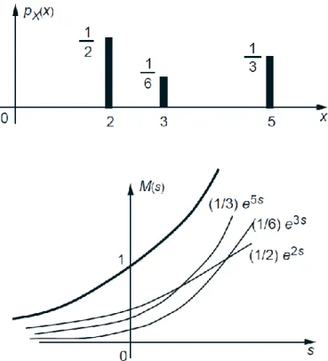
Example 1. Let
Then, the corresponding transform is
.
Figure 1: The PMF and the corresponding transform for Example. The transform consists of the weighted sum of the three exponentials shown. Note that at , the transform takes the
value . This is generically true since
.
It is important to realize that the transform is not a number but rather a function of a free variable or parameter . Thus, we are dealing with a transformation that starts with a function, e.g., a PDF (which is a function of a free variable ) and results in a new function, this time of a real parameter . Strictly speaking, is only defined for those values of for which
is finite.
From Transforms to Moments
The reason behind the alternative name “moment generating function” is that the moments of a random variable are easily computed once a formula for the associated transform is available. To see this, let us take the derivative of both sides of the definition
with respect to . We obtain
.
This equality holds for all values of . By considering the special case where , we obtain†
.
More generally, if we differentiate times the function with respect to , a similar calculation yields
.
†This derivation involves an interchange of differentiation and integration. The interchange turns out to be justified for all of the applications to be considered in this course. Furthermore, the derivation remains valid for general random variables, including discrete ones. In fact, it could be carried out more abstractly, in the form
,
leading to the same conclusion.
Example 2. We saw earlier (Example 1) that the PMF
has the transform
.
.
Inversion of Transforms
A very important property of transforms is the following.
Inversion Property
The transform completely determines the probability law of the random variable . In particular, if for all , then the random variables and have the same probability law.
Sums of Independent Random Variables
Transform methods are particularly convenient when dealing with a sum of random variables. This is because it turns out that addition of independent random variables corresponds to multiplication of transforms.
Let and be independent random variables, and let . The transform associated with is, by definition,
.
Consider a fixed value of the parameter . Since and are independent, and are independent random variables. Hence, the expectation of their product is the product of the expectations, and
.
By the same argument, if is a collection of independent random variables, and
,
then
Summary of Transforms and their Properties
The transform associated with the distribution of a random variable is given by
The distribution of a random variable is completely determined by the corresponding transform.
Moment generating properties:
, , .
If , then .