Draft JEBO 07-2018.pdf

(1)

Competing Currencies in the Laboratory

∗

Janet Hua Jiang†

Bank of Canada

Cathy Zhang‡

Purdue University

This version: July 2018

Abstract

We investigate competition between two currencies as a result of decentralized interactions between human subjects. We design a laboratory experiment based on a simple two-country, two-currency search model to study factors that affect circulation patterns and equilibrium se-lection. Experimental results indicate foreign currency acceptance rates decrease with relative country size but are not significantly affected by the degree of integration. Subjects tend to al-ways accept both currencies even though rejecting either currency is consistent with equilibrium. Introducing government transaction policies biased towards domestic currency significantly re-duces the acceptability of foreign currency. These findings suggest government policies can serve as a coordination device when multiple currencies are available.

JEL Classification: C92, D83, E40

Keywords: currency competition, multiple currencies, macro experiments

∗

We are grateful to two anonymous referees, Gabriele Camera, Tim Cason, John Duffy, Daniela Puzzello, Guil-laume Rocheteau, Julian Romero, Yaroslav Rosokha, Randy Wright, and Yu Zhu for helpful discussions and com-ments. We also thank conference and seminar participants at the 2018 Canadian Economics Association Meeting in Montreal, the 2017 8th BESLab International Workshop on Experimental Macroeconomics in Stonybrook, 2016 ESA North American Meetings in Tucson, 2015 ESA World Meetings in Sydney, Purdue University, and the Bank of Canada for feedback. We gratefully acknowledge funding support from the Bank of Canada. Chineze Christopher, Stanton Hudja, and Benjamin Raymond provided excellent research assistance. The views expressed in this paper are those of the authors. No responsibility for them should be attributed to the Bank of Canada. There are no declarations of interest to report.

†

Address: Bank of Canada, 234 Wellington Street Ottawa, ON, K1A 0G9, Canada. E-mail: [email protected]

‡

(2)

1 Introduction

Government-issued money, ornational currency, is the most widely used currency in most modern economies and has an important role as a generally accepted medium of exchange. Historically, the first known paper currencies were issued by local governments and tended not to circulate beyond a region’s borders. Only thereafter did the secondary use of paper currencies from other localities’ become more common and often times at a lesser scale (Ferguson 2009). While only one or a fewinternational currencies tend to widely circulate at given point in time, their general acceptance raises the question of whether another currency can substitute or crowd out the use a national currency. More recently, the dominance of national currencies has received renewed interest among policymakers as privately issued cryptocurrencies, such as bitcoin, have started being used alongside government-issued money. What determines which currency out of many potential candidates emerges as a universally accepted payment? And how are circulation patterns affected by government policy?

In this paper, we investigate competition between multiple currencies using experimental meth-ods and examine how various features of the economy affect their roles in exchange. The start-ing point of our analysis is the two-country, two-currency search model of Matsuyama, Kiyotaki, and Matsui (1993), where domestic and foreign currency compete and can circulate as media of exchange. Search theoretic models are particularly well suited for studying the use of multiple currencies since these models endogenously generate different payment regimes, without having to restrict which currencies private citizens can accept. For that reason, we adopt a version of Matsuyama, Kiyotaki, and Matsui (1993) in the laboratory to study the circulation pattern of the two currencies and investigate how they are affected by economic integration, relative country size, and government policies favoring domestic currency.

(3)

for either home or foreign currency.

Since the circulation of token objects is driven by both fundamentals and beliefs regarding what other agents do, there are multiple equilibria that differ in the areas of circulation of the two currencies. One equilibrium features only local circulation of currencies. In another equilibrium, one currency is internationally accepted while the other remains local. Finally, there is also an equilibrium where both currencies are everywhere accepted. Whether there are zero, one, or two international currencies depends on the fundamentals of the economy, such as country size and degree of economic integration, as well as expectations regarding what other agents do. While the multiplicity of equilibria poses predictive challenges for the theory, our experimental approach can help discern which equilibrium is selected in the laboratory.1 Equilibrium selection is therefore an important reason we go to the laboratory.

There are several other advantages of using an experimental approach to study multiple cur-rencies. First, there is lack of micro-level data on the circulation of multiple currencies, which makes empirical studies using field data sparse.2 Second, experimental methods give clean control of the environment and allow us to isolate the factors that drive acceptance decisions. Third, we directly observe currency acceptability and can incentivize subjects in the laboratory. Field data often rely on surveys susceptible to errors due to insufficient incentives for truthful or careful re-porting, misunderstandings about the survey questions, etc. Finally, it is possible to conduct policy experiments and counterfactuals in the laboratory that are not feasible to implement in practice.

In our benchmark experiment, we implement a simple version of the model in the laboratory and investigate whether agents who have access to two intrinsically worthless tokens coordinate on an equilibrium with zero, one, or two currencies everywhere accepted. Our design allows us to explore how the degree of economic integration and relative group size matter for currency circulation and equilibrium selection. In the model, these two parameters affect the matching process and hence the likelihood that individuals expect to meet foreigners relative to compatriots.

We introduce three treatments as part of the benchmark design. The baseline treatment features symmetric country sizes and a high level of integration, the second has a lower level of integration and keeps country sizes symmetric, and the third has different country sizes. Results indicate the

1

A different approach to equilibrium selection is the evolutionary approach to study how agents coordinate on an equilibrium; see Matsuyama, Kiyotaki, and Matsui (1993) and Wright (1995) in the context of monetary search models.

2

(4)

degree of integration has no significant effect on currency circulation. With asymmetric country sizes, subjects from the larger country show stronger home bias and reject foreign currency more frequently compared with subjects in the baseline treatment. In all three treatments, the experi-mental economies are close to the unified currency regime with low rejection rates for both home and foreign tokens.

We next extend our design to incorporate government transaction policies biased towards do-mestic currency. This captures the role of government policies and legal tender laws that aim to increase the acceptance of local money. The basic idea is that by simply accepting a particular currency in its own trades, governments may induce private agents to do the same. We find the pres-ence of government agents coordinates subjects towards rejecting foreign tokens more frequently. The foreign token rejection rate increases on average from 7% in the baseline treatment to 57% with government transaction policies. On the other hand, home token rejection rates remain similar to the baseline treatments without government. These results suggest government policies biased towards domestic currency can act as a coordination device, consistent with the role of government transaction policies in practice.

The rest of the paper proceeds as follows. Section 2 discusses related literature and our contri-bution. Section 3 describes the theoretical framework used for the experiments. Section 4 describes the experimental design and provides a broader discussion on some modeling and design choices. Section 5 reports the main results and discusses robustness. Section 6 concludes.

2 Related Literature

(5)

(2014) and Duffy and Puzzello (2014) study monetary exchange versus gift giving when good outcomes can be supported without money through social norms. Their findings suggest that money acts as a coordination device even when it is not theoretically essential for trade. Camera, Casari, and Bortoletti (2016) and Arifovic, Duffy, and Jiang (2017) study competing payment methods linked to the same currency, with a focus on the effect of the cost and reward structure of different payment methods.

This paper has two key differences from this previous work. First, our experiment studies the circulation patterns of two currencies, rather than competition between multiple commodity monies, commodity money versus currency, gift giving versus fiat money, etc.3 Second, we consider an asymmetric matching process where two groups are distinguished by the matching function. This distinction defines an individual’s nationality or group membership, a key aspect affecting currency regimes in practice.

The closest papers to ours are Rietz (2017) and Ding and Puzzello (2017), which were both written concurrently with ours. Rietz (2017) studies the acceptance of a secondary currency when a primary currency already circulates based on the dual currency economy of Craig and Waller (2000). Rietz’s focus is on the choice to accept the secondary currency given the acceptability of another currency, while we focus on competition between two currencies, distinguish between groups as a result of matching, and introduce a different type of government policy biased towards home currency. Ding and Puzzello (2017) also study competition between two currencies but use the divisible money model of Zhang (2014). Our simpler set-up with indivisible money and goods provides a benchmark that focuses exclusively on the acceptability decision, without having to deal with terms of trade and prices, which may also affect acceptance decisions. While Ding and Puzzello (2017) do not study the impact of economic integration and relative country size as in this paper, they focus two types of policy interventions – government transaction policies, similar to this paper, and information costs on foreign currency acceptance decisions. Our findings are therefore complementary to each other and together offer a more comprehensive picture of the factors (e.g., integration, size, government policies, circulation of a primary currency, information costs, etc.) driving circulation patterns in dual currency economies.

3

(6)

3 Theoretical Framework

Our experimental economy is based on a simplified version of the two-country, two-currency search model of Matsuyama, Kiyotaki, and Matsui (1993). We first describe the baseline model without government transaction policies in Section 3.1, and then introduce these policies in Section 3.2. Section 3.3 briefly discusses the model’s welfare implications.

3.1 Baseline Model without Government Policy

Time is discrete and continues forever. Agents are divided into two groups, or “countries,” called Red and Blue. The measure of agents in country i∈ {r, b} is ni, where 2n= nr+nb is the total size of the economy. All agents have a discount factor across periods of β = 1/(1 +r) ∈ (0,1), wherer >0 is the discount rate.

Countries are defined by a pairwise matching technology where a pair of agents from the same country are more likely to be matched than a pair of agents from different countries. Table 1 summarizes agents’ matching probabilities, where entries give αij, the probability an agent from countryimeets an agent from j. The matching process depends on country sizes,nr and nb, and the parameter,ρ∈[0,1], which captures the degree of integration between countries. Other things being equal, it is more likely to meet someone from the larger country. Asρ→1, the two countries become more integrated, whileρ= 0 implies the two economies are closed and do not interact with one another.

Table 1: Meeting Probabilities

Red Agent Blue Agent

Red Agent αrr= nr nr+nb +

(1−ρ)nb

nr+nb αrb= ρnb nr+nb

Blue Agent αbr= _n_rρn₊r_n_b αbb= _n_rn₊b_n_b +(1_n−_r₊ρ)_nn_br

There are three indivisible objects in the economy: a consumption good and two tokens labeled by color, red and blue. Each agent costlessly produces a different variety of the consumption good but does not want to consume it. Instead, agents get flow utilityu >0 only from consuming another agent’s variety.4 Immediately following consumption, agents produce a unit of good at no cost and

4

(7)

carry it to the next period. Tokens are intrinsically worthless: they cannot be consumed or used for production. Their roles in the economy is to serve as tangible media of exchange. Following Matsuyama, Kiyotaki, and Matsui (1993), agents must use one of the tokens to exchange for their consumption good. This assumption rules out barter, credit, and gift-giving arrangements, which allows us to focus on the competition between two currencies as alternative means of payment.5

Agents can hold at most one object: one unit of good or one unit of a red or blue token. A fraction Mi ∈ (0,1) of agents (buyers) in country i are initially endowed with an indivisible unit of their home currency, of which there is a constant per capita supply.6 The remainder (1−Mi) of agents (sellers) are initially endowed with one unit of good. We assume currency trading is not allowed.

The above modelling assumptions reduces agents’ action space and simplifies their decisions. In particular, there are only gains from trade between an agent with currency (buyer) and an agent with good (seller). When a buyer and a seller meet, they indicate simultaneously whether or not they want to trade. If both agree, they exchange inventories one for one; otherwise, no trade occurs. Following trade, agents’ roles as buyers and sellers are reversed: a buyer immediately consumes the good, earning utilityu >0, produces one unit of good at no cost and becomes a seller in the next period; similarly, the new owner of currency becomes a buyer.

3.1.1 Monetary Equilibrium

The state of the economy is fully characterized by the distribution of tokens. At each point in time, there will be some agents with one unit of money each (buyers) and a disjoint group with no money (sellers). Letmik denote the fraction of buyers from countryiwith currencyk andmi0 denote the

fraction of sellers in country i. Since currency is indivisible, the condition

mi0+mir+mib= 1

must be satisfied, where the vector m = (mij) describes the asset distribution across agents. In addition, the aggregate supply of currency iin countryimust equal its aggregate demand:

niMi=nimii+njmji. 5

Without the assumption that agents must use tokens to buy their consumption good, the model would allow for nonmonetary arrangements such as gift exchange, sustained through community enforcement as in Kandori (1992) and Aliprantis, Camera, and Puzzello (2006).

6

(8)

Following Matsuyama, Kiyotaki, and Matsui (1993), we focus on symmetric stationary equilibria in pure strategies, where agents from the same country follow the same pure strategy and asset distributions are constant over time. Notice a buyer matched with a seller will always want to trade. In what follows, we consider different types of equilibria based on which currencies sellers accept. To simplify the presentation, we focus on candidate equilibria where agents always accept their home currency.7 _{The key issue is then whether trade occurs when a seller from} _i _meets

a buyer with foreign currency j 6= i. Let λi = 1 if the seller in country i accepts currency j (both domestic and foreign currency circulates in country i) and λi = 0 if the seller rejects currency j (only domestic currency circulates in countryi). The regimes we focus on are given by λ≡(λr, λb) ={(0,0),(0,1),(1,0),(1,1)}.

We call a currency a national currency if it is only accepted by sellers from that country and a international currency if it is accepted by all sellers. Hence, an equilibrium with two national cur-rencies (no international currency) corresponds toλ= (0,0), an equilibrium with one international currency corresponds to λ= {(0,1),(1,0)}, and an equilibrium with two international currencies corresponds to λ= (1,1).

When agents of different nationality meet, the stationary distribution of currency holdings satisfies

αij(mi0mji−miimj0λj) = 0, (1) αij(mi0mjjλi−mijmj0) = 0. (2)

These expressions use the fact that trade between agents of the same nationality do not changem since the aggregate distribution will not be affected. According to (1), when a seller fromimeets a buyer fromjwith currencyi, the amount of currencyiin countryi,mii, will increase. At the same time, when a buyer from i with currency i meets a seller from j, mii will decrease if the agents decide to trade (λj = 1). In a stationary equilibrium, this net change must be zero. A similar explanation applies to (2).

Consequently, the stationary asset distributionm satisfies

mi0mji

| {z }

outflow of currencyifrom countryj

= miimj0λj

| {z }

inflow of currencyito countryj

, (3)

7

(9)

mi0mjjλi

| {z }

inflow of currencyjto countryi

= mijmj0

| {z }

outflow of currencyjfrom countryi

. (4)

According to (3), the flow out of currency i from country j must equal the flow in of currency i to country j. Similarly, (4) says the inflow of currency j to country i must equal the outflow of currency j from i.

LetVi0 denote the lifetime utility of a seller from countryiwho holds no money andVik denote the lifetime utility of a buyer from country iwho starts a period with currency k. The flow value of being a seller from countryican be written as

rVi0 = (αiimii+αijmji)(Vii−Vi0)

| {z }

exp. trade surplus when seller meets buyer with local money

(5)

+ (αiimij+αijmjj)λi(Vij−Vi0)

| {z }

exp. trade surplus when seller meets buyer with foreign money

.

Equation (5) consists of the probability a seller from i meets a local or foreign buyer holding currency itimes the trade surplus in that meeting, plus the probability the seller from i meets a local or foreign buyer holding currencyj.

The flow value of a buyer from iholding domestic currency is

rVii= (αiimi0+αijmj0λj)(u+Vi0−Vii)

| {z }

exp. trade surplus of buyer with local money in local and foreign meetings

. (6)

Similarly, the flow value of being a buyer from iholding foreign currency is

rVij = (αiimi0λi+αijmj0)(u+Vi0−Vij)

| {z }

exp. trade surplus of buyer with foreign money in local and foreign meetings

. (7)

Equation (6) is the flow value of being a buyer from country i holding domestic currency, which consists of the probability the buyer meets a domestic or foreign seller times the gains from trading. Similarly, equation (7) is the flow value of being a buyer from country iholding foreign currency, which is the probability a buyer meets a domestic or foreign seller times the gains from trading. In (6) and (7), the value of obtaining the consumption good is u+Vi0: one gets direct utility from

consumption (u) plus the value of being a seller (Vi0) since acquiring a consumption good enables

the agent to produce next period.

(10)

always accept their domestic currency, we just need to verify the seller is willing to accept foreign money. In that case, the incentive compatibility conditions for a seller from country iare

λi =







1 ∈[0,1]

0

ifVij







> = <

Vi0. (8)

According to (8), a seller is willing to accept foreign currency if the value of holding it and becoming a buyer exceeds the value of remaining a seller. For him to reject foreign money, the opposite condition must hold.

3.1.2 Currency Regimes

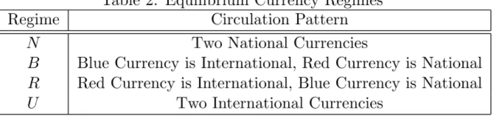
Acurrency regime is a stationary and symmetric equilibrium, (λ,m,V), satisfying conditions (3)– (8). Table 2 summarizes the currency regimes that may emerge (recall we focus on equilibria where agents always accept home currencies). For each regime, we solve equations (3)–(7) and check the conditions in (8) are satisfied. If so, then the candidate regime constitutes an equilibrium.

Table 2: Equilibrium Currency Regimes

Regime Circulation Pattern

N Two National Currencies

B Blue Currency is International, Red Currency is National R Red Currency is International, Blue Currency is National

U Two International Currencies

Regime N: Two National Currencies. In this equilibrium, sellers never accept foreign cur-rency: i.e., λ = (0,0). We call this Regime N. Since only local currency circulates, mrr = Mr, mbb =Mb, and mrb=mbr = 0. The value functions simplify to

rVi0 =αiiMi(Vii−Vi0),

rVii=αii(1−Mi)(u+Vi0−Vii), rVij =αij(1−Mj)(u+Vi0−Vij).

We now verify a seller’s incentive condition to never accept foreign currency, orVij ≤Vi0. This

will be the case if

αij ≤

α2_iiMi(1−Mi) (r+αii)(1−Mj)

(11)

An equilibrium with two national currencies exists so long asαij is small enough: if one does not come across foreigners too often, then it is optimal to reject foreign money. Equation (9) also gives the existence condition for Regime N in terms of the degree of integration ρ and the size of Red, nr. For a given country size, a sufficiently open economy would eliminate this equilibrium since a higherρincreases the probability of encountering foreigners and thus the incentive to accept foreign money.

Regimes R and B: One International Currency, One National Currency. The emergence of an international currency occurs when sellers from one country accept both currencies. Here we focus on the case where sellers from Red accept both currencies, while sellers from Blue only accept domestic money, i.e. λ = (1,0). We call this Regime B. In that case, the blue token emerges as the sole international medium of exchange. Since the red token only circulates at home: mrr=Mr and mbr = 0. The fraction of blue tokens held in Red and Blue, respectively, are given by

mrb=

(1−Mr)Mb 1 +αbr

αrb(1−Mr) ,

mbb= Mb

1 +αbr

αrb(1−Mr) .

For citizens from Red, the value functions are

rVr0 = αrrmrr(Vrr−Vr0)

| {z }

exp. trade surplus when seller meets buyer from Red with red token

+ (αrrmrb+αrbmbb)(Vrb−Vr0)

| {z }

exp. trade surplus when seller meets buyer with blue token

,

rVrr = αrrmr0(u+Vr0−Vrr)

| {z }

exp. trade surplus of buyer with local money in local meetings

,

rVrb= (αrrmr0+αrbmb0)(u+Vr0−Vrb)

| {z }

exp. trade surplus of buyer with blue token in local and foreign meetings

.

For citizens from Blue, the value functions are

rVb0= (αbrmrb+αbbmbb)(Vbb−Vb0),

(12)

In this equilibrium,Vib> Vi0, which guarantees that sellers from both countries have an incentive

to accept the blue token. Next, to ensure that sellers from Red are willing to accept the red token, Vrr≥Vr0 must hold, which requires

αrrmr0(r+αrrmr0+αrbmb0)≥αrbmb0(αrrmrb+αrbmbb).

Finally, sellers from Blue will not accept the red token if Vbr ≤Vb0, which requires

αbrmr0(r+αbamr0+αbbmb0)≤αbbmb0(αbamrb+αbbmbb).

Intuitively, these conditions require that it be relatively easy for a buyer from Red to find a Red seller, but relatively hard for a Blue buyer to find a Red seller.

Regime U: Two International Currencies. An equilibrium with two international currencies, λ= (1,1), occurs when sellers from both countries accept both currencies. We call this RegimeU. The value functions in this regime are

rVi0 = (αiimii+αijmji)(Vii−Vi0) + (αiimij +αijmjj)(Vij−Vi0),

rVii= (αiimi0+αijmj0)(u+Vi0−Vii),

rVij = (αiimi0+αijmj0)(u+Vi0−Vij).

For Regime U to exist, we must have Vii = Vij, so that buyers are indifferent between holding currency i and currency j 6= i. Consequently, the two monies are perfect substitutes. Since Vii> Vi0 is always satisfied, this regime always constitutes an equilibrium.

(13)

3.2 Model with Government Transaction Policies

An idea dating back to Smith (1963) and Lerner (1947) is that by accepting a particular currency in its own transactions, governments can induce private citizens to do the same. We examine this idea and introduce a group of traders similar to the government agents in Aiyagari and Wallace (1997) and Li and Wright (1998), who follow an exogenously specified trading rule regarding which currency they accept as payment, rather than choosing to accept a currency based on optimizing behavior. Specifically, we assume there is a constant fraction gb ∈ [0,1] of government agents in the Red group and a constant fractiongb ∈[0,1] in the Blue group.

As before, there are two currencies – a red token and a blue token – that are identical except for their initial distributions. Government agents consume and produce like private agents and are subject to the same matching process. However, in contrast with private agents who adopt trading strategies based on maximizing behavior, government agents follow exogenous trading rules called government transaction policies. In what follows, we consider a benchmark policy where government agents only accept domestic currency in exchange for goods (when a seller), and always accept goods for any currency (when a buyer).

As before, we define currency regimes in terms of the acceptance decisions of private sellers. Hence we continue to call Regime U an equilibrium where both currencies are accepted by private sellers, even though government sellers never accept foreign currency by assumption. The full model set up and details of the analysis of the currency regimes that arise are in Appendix A. Here we summarize the key predictions.

(14)

3.3 Welfare

We now briefly discuss the model’s welfare implications in terms of steady state welfare in the two countries. In general, welfare rankings across regimes are sensitive to the parameterization, but we can make a few general statements assuming equal money supplies, i.e. Mr=Mb.

1. Welfare is highest in Regime U for both countries.

2. Welfare is higher in Regime R (B) than Regime N for the Red (Blue) country.

3. Welfare is higher in the larger country in Regimes N and U.

4 Experimental Design

We now describe our implementation of the model environment in the laboratory. We first dis-cuss our choice of parameters for the experiment, and then describe the experimental procedure. Additional details of the design are in Appendices B–E.

4.1 Parameterization

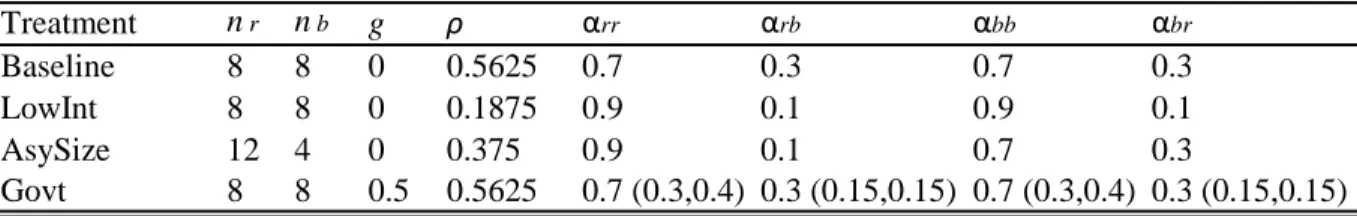
Our experiment follows a between-subjects design where each session consists of a new group of subjects making decisions under a single parameter set. We have four treatments: (1) Baseline, (2) LowInt, which captures the effect of economic integration, (3) AsySize, which captures the effect of relative country sizes, and (4) Govt, which investigates the effect of government transaction policies that favor acceptance of home token. Table 3 summarizes the model parameters used in each treatment. These parameters are chosen to imply the coexistence of RegimesN,R,B andU, as shown in Figures 1 and 2.

(15)

gr = gb = 0.5).8 All other parameters are set to the same values as in the Baseline treatment. The parameter values for each treatment are summarized in Table 3. Table 4 compares welfare across regimes, treatments, and groups. Consistent with Section 3.3, we see welfare is the highest in Regime U for each treatment.

In the following, we discuss in more detail two features of our experimental design and discuss their implications.

Finite Population Our experimental study involves a finite number of subjects, different from the continuum of agents in the theoretical model. Since an individual is non-atomistic in a finite population and can affect the aggregate asset distribution, we follow Duffy and Ochs (2002) and check all four types of equilibria exist with a finite population for each parameter set (see Appendix C for more details). In particular, we simulate the asset distribution assuming all agents follow the equilibrium strategy and compare with the asset distribution assuming that a single agent follows each of all possible deviation strategies while all other agents follow the equilibrium strategy. We then verify the existence of each of type of equilibrium by showing the individual’s lifetime utility is maximized by following the equilibrium strategy, or that unilateral deviations from the equilibrium strategy are not profitable using the asset distributions derived from the simulations.

Finite Horizon Our theoretical model in Section 3 features an infinite horizon where all agents have a constant discount factor β ∈ (0,1). The standard approach to implementing an infinite horizon in the laboratory follows Roth and Murnighan (1978) where after each period, the experi-mental economy continues with a fixed probability set equal toβ ∈(0,1). Hence, the experimental economy is terminated with probability 1−β. For our experiment, we implement the infinite hori-zon model instead with a large finite number of periods. Specifically, each session of the experiment lasts for a fixed 150 periods, which all subjects are fully informed of. In the following, we explain the main reasons for this design choice and discuss alternative approaches.

First, a fixed horizon ensures against short sequences, which is critical in our setting. Since subjects are initially endowed with either the consumption good or home token, a long trading sequence is required to give a chance for both tokens to circulate across groups. If the trading

8_{We set}_g

r=gbto keep the parameterization symmetric across groups to be more comparable with the Baseline

treatment, which features a symmetric parameterization across groups. Regarding the magnitude of (gr, gb), too high

values will get rid of the three regimes with international currencies, while too low values may make the presence of government agents not salient enough to subjects. We therefore chosegr=gb= 0.5 since it is salient and admits all

(16)

horizon is too short, subjects will have only limited, or even no, encounters with the foreign token. With real random termination where random sequences are drawn in real time, there is no guarantee against short sequences even if the continuation probability is close to one. There is also the concern that, especially with β close to one, the experiment will continue beyond the time frame subjects are recruited for.

Using predrawn sequences to allow a more commensurate comparison of acceptance rates across sessions and treatments is another alternative but raises additional concerns. The choice of a particular sequence could be arbitrary and subjective. In addition, using predrawn sequences may introduce uncertainty about the length of the experiment among subjects, an unintended consequence and deviation from the original model with infinite horizon and discounting. Using a long fixed horizon alleviates both these issues.

The typical and main argument against implementing a monetary model in the laboratory with a fixed horizon is that it eliminates monetary equilibria by backward induction. This is a valid concern in view that McCabe (1989) finds players learn not to hold money near the end of the finite horizon (of six periods). We think the seriousness of this concern is sufficiently contained for our experiment for the following reasons. First, our experiment lasts for 150 periods, which is a very long fixed horizon. As suggested by Osborne and Rubinstein (1994), subjects who play a game with a long fixed horizon may ignore the existence of the finite horizon until the very end of the game, and for most of the experiment, their strategic thinking may be more representative of a game with an infinite horizon. Second, the typical concern that a fixed horizon eliminates monetary equilibria is less of a worry in our study. Since we assume production is costless, there is no strict incentive to not produce even when the game is about to end. This sustains monetary equilibria since agents need to use one of the two currencies in order to consume.9 We recognize costless production does not rule out other equilibria: in the final period, sellers are indifferent between trading and not and could in principle choose to trade with any probability. This however did not materialize in our experiment. We investigate how subjects’ choices at the end of the game affect earlier decisions

9

(17)

and find the effect is statistically insignificant and the magnitude is very small (see Tables D3 and D4 in Appendix D).

To validate our argument above, we ran pilot sessions comparing a fixed horizon versus indefinite horizon design. We ran two sessions with a fixed 100 periods and three sessions with an indefinite horizon under random termination.10 In the latter, subjects were instructed the number of periods was determined by a random termination device such that there was a β = 99% chance the experiment would continue to another period. We used predrawn random sequences where the three sessions lasted for 110, 116, and 102 periods, respectively.

Relative to fixed horizon sessions, we find the indefinite horizon sessions feature higher token rejection rates, more heterogeneity across subjects’ actions, and therefore noisier aggregate results. Specifically, the foreign (home) rejection rate for the three indefinite horizon sessions (averaged across subjects) was 16.1% (6.6%), versus 4.2% (3.7%) for the two definite horizon sessions.11 The standard deviation of the foreign- (home-) token rejection rate was 24.5% (16.1%) for the indefinite horizon sessions, compared with 7.1% (6.3%) for the fixed horizon sessions. These results reassure us that a long fixed horizon is a reasonable choice for our experiment. For instance, we would expect to see higher rejection rates for the finite horizon sessions if there were end-of-period effects; the fact that we observed the opposite helps alleviate this concern. The higher rejection rates and noisier results from the indefinite horizon sessions also seem to validate our concern that this design may induce uncertainty about the length of the experiment, an unintended consequence and deviation from the original model with infinite horizon and discounting.

4.2 Experimental Procedures

All experimental sessions in this study were conducted at the Vernon Smith Experimental Eco-nomics Laboratory at Purdue University in 2016 and 2017. Participants were undergraduate stu-dents at Purdue University, recruited through the Online Recruitment System for Economics Ex-periments. No subject participated in more than one session of the project, although some subjects participated previously in other economics experiments run by other researchers. The total length of a session ranged from 50 to 80 minutes. Participants received a $5 participation payment plus 10_{The design of the pilots is similar to the Baseline treatment except the probability of meeting a foreigner, set to} 0.25, is slightly lower than the value of 0.3 used in the Baseline treatment (we chose 0.3 for the final design since it is slightly easier to communicate to subjects, especially in the AsySize treatment). We also increased the duration of the experiment from 100 to 150 periods to get more observations.

11

(18)

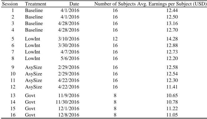
earnings from the experiment. Table 5 summarizes session information including average earnings per subject. See Appendix E for the experimental instructions for the Govt treatment.

Each session consisted of instructions, a follow-up quiz on the instructions, and the experiment. Upon entering the laboratory, participants were randomly assigned a computer station and given a written copy of the instructions. The instructions were then read out loud by the experimenter to reinforce common knowledge of the environment. Participants then completed a short quiz about the instructions. After completing the quiz, the experimenter went over the correct answers, answered questions, collected the quiz, and began the experiment. All parts of the experiment were programmed with z-Tree (Fischbacher 2007).

Each session of the experiment consists of 150 periods of bilateral interactions with random matching. Participants are divided into one of two groups, Red or Blue, of potentially different sizes. Group membership is randomly assigned and remains fixed throughout the session. Each participant is initially endowed with one unit of a consumption good (called “corn” in the ex-periment), one unit of a blue token, or one unit of a red token. Hence an individual’s role as a buyer or seller in the first period is exogenous and determined by random assignment; however, in subsequent periods, an individual’s role as buyer or seller is endogenously determined by trading outcomes in the previous period.

While tokens are intrinsically worthless objects and cannot be redeemed for points, holding corn yields positive points if and only if one obtains it from someone else. To receive points, individuals must trade either a blue or red token for corn. The instructions also emphasized that it may take more than one period to obtain corn from another participant. Since tokens and corn are indivisible, exchanges are one for one. Participants are induced to maximize their earnings in points, which are converted into U.S. dollars and paid out at the end of the experiment. The exchange rate for all sessions is 1 point = $0.02.

At the start of each period, a random matching process pairs an individual subject with a partner. All participants are informed of the ex ante meeting probabilities in the instructions. As in the model, the probability an individual is paired with someone from their own group is greater than the probability of being paired with someone from the other group. These probabilities differ across treatments. For instance, in the AsySize treatment, subjects are instructed:

In each period, you may either be matched with someone from your own group, or someone

(19)

• If you are in Group Red, there is a 90% chance you will be paired with someone else from Group Red and a10% chance you will be paired with someone from Group Blue.

• If you are in Group Blue, there is a 70% chance you will be paired with someone else from Group Blue and a30% chance you will be paired with someone from Group Red.

These probabilities will remain the same throughout the experiment and will appear on your

computer screen.

Once matched, both parties find out their partner’s good. If one subject holds corn and the other holds a token, the pair is simultaneously asked in isolation whether they would like to exchange inventories with their partner. Trade occurs if and only if both parties agree, and only someone who successfully trades for corn will be awarded points. If trade occurs, each subject begins the next period holding their partner’s good from the previous period. If both subjects hold corn or both hold tokens, they are informed about each others’ inventories; no trade occurs and they carry their current inventory into the next period. Subjects are then rematched for the next period and asked again if they would like to trade. Figure 3 summarizes the timing of the experiment, and Figure 4 provides a sample screenshot of the trading screen for the Govt treatment.

5 Experimental Results

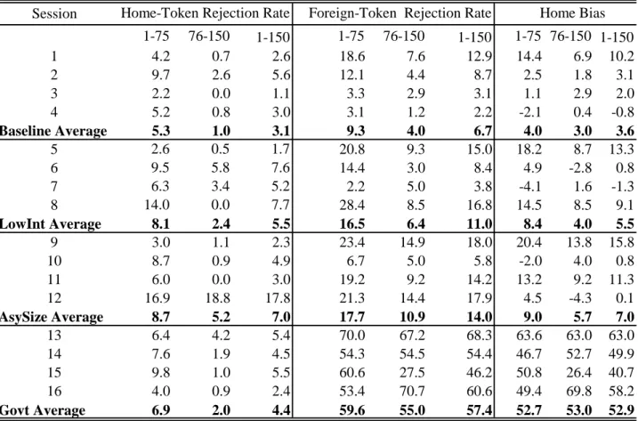
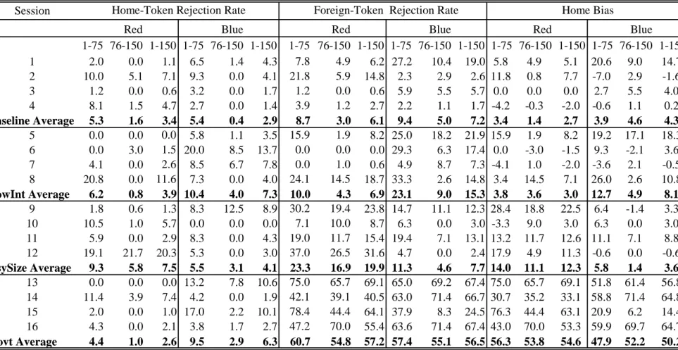
We now report the main findings from the experiments. Table 6 and 7 report summary statistics for aggregate home and foreign token rejection rates. For each session, the home (foreign) token rejection rate is computed as the ratio between the number of home (foreign) token-corn meetings and the number of rejections in those meetings. We also compute the degree of home bias in each session, defined as

Home Bias = % Foreign Token Rejections −% Home Token Rejections.

In the tables, we provide treatment-level statistics as the average of the four sessions in the treat-ment. To gain some insight about the time trend of the three variables, we report the statistics for the entire session, along with the first and second halves of the session.

(20)

Since there are only a small number of observations for the rank-sum tests on the session level statistics, we complement these tests with analysis of individual choices. Specifically, we run probit regressions with random effects on individual subjects’ decisions on whether or not to reject a home or foreign token in a token-corn meeting. We run three sets of regressions: the first set uses observations of home token-corn meetings to analyze home token acceptance decisions, the second uses observations of foreign token-corn meetings to study the foreign token acceptance decisions, and the third uses all token-corn observations to study the degree of home bias. Each set of regressions includes 15 specifications. The first three use pooled data from all four treatments with observations for all subjects, and subjects in the Red and Blue group, respectively. The remaining 12 specifications use data from the individual treatments.

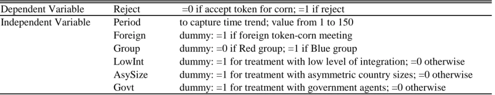
Variables in the probit regressions are summarized in Table 9. The dependent variable is “Re-ject” which equals 1 if the token is rejected, and 0 otherwise. To study how token rejection rates change over time, we include a time trend of the rejection rate with the variable “Period” in the first two sets of regressions. The effects of integration, asymmetric country sizes, and govern-ment transaction policies are captured respectively by the coefficients on “LowInt,” “AsySize,” and “Govt.” The same variables appear in the third set of regressions; in addition, we include product terms of these variables multiplied by “Foreign.” The time trend of home bias is captured by the coefficient on “Period x Foreign.” The effect of the treatment variables on home bias is captured by the product terms “LowInt x Foreign,” “AsySize x Foreign,” and “Govt x Foreign.” Regression results are summarized in Tables 10–12. For each variable, we report its marginal effects on the percentage of token rejections and standard errors clustered at the session level.12

We organize the discussion of the experimental results in the following findings.

Finding 1 (Home-Token Rejection Rate). In all treatments, the home-token rejection rate is low and decreases over time for both groups. The rejection rate is not significantly affected by any of the treatment variables.

The home rejection rate averages 3.1% for the Baseline treatment, 5.5% for the LowInt treat-ment, 7.0% for the AsySize treattreat-ment, and 4.4% among human subjects in the Govt treatment.

12

(21)

Table 6 also shows the home rejection rate decreases from the first half to second half of the exper-iment for all four treatments. The regression results in Table 10 are consistent with this decreasing trend. As seen from the rank-sum tests in Table 8 and the probit regressions in Table 10, we do not find any significant effect of the treatment variables on the home token rejection rate.

Finding 2 (Home Bias). Subjects’ decisions exhibit systematic home bias across treatments and groups. Home bias tends to dissipate over time in the treatment without government transaction policies, but persits in the Govt treatment.

The experimental data shows the presence of home bias in all four treatments and for both groups (see Tables 6, 7 and 12). The probit regression for home bias using pooled data across the four treatments indicates the rejection rate for foreign tokens is 7.3% higher than for home tokens (see Table 12a).

In the treatments without government agents, notice the two tokens are identical except that they are associated with a different group in terms of color and are held initially by the group labeled the same color. This color association may have created a sense of “national” identity among some subjects, inducing them to favor home tokens over foreign tokens.13 At the end of the experiment, we ask subjects in a questionnaire whether they rejected a foreign token and if yes, why. The most frequent answer is that they wanted to keep corn within their own group. This home bias, though present, seems to weaken over time, consistent with the negative coefficient for the term “Period x Foreign” in the probit regression. In the Govt treatment, there is an additional and more substantial source of home bias: the existence of government agents reduces the acceptability of foreign tokens and therefore the value of holding them. In that treatment, home bias is more persistent and does not taper off over time.

In the next three findings, we discuss how the treatment variables affect the foreign token rejection rate and home bias.

Finding 3 (Effect of Integration on Foreign-Token Rejection Rate and Home Bias). A lower degree of integration has a weak positive effect on the foreign-token rejection rate and the degree of home bias, both of which attenuate over time.

13

(22)

Relative to the Baseline treatment, Tables 6 and 7 show the rejection rate for foreign tokens and the degree of home bias are higher for the LowInt treatment, which features a lower probability of meeting a foreigner than the Baseline treatment. However, the differences between the Baseline and LowInt treatment are small in magnitude and statistically insignificant, as seen in Tables 11 and 12.

In the real world, we often observe people residing along the geographical border between two countries are often more willing to accept foreign currency due to frequent encounters with foreigners, which seems to contradict the result from our experimental study. A possible reason that the effect of economic integration is not as salient in our study could be because the extent of economic integration has more aspects than what we capture in our experiment, such as the recognizability of the foreign currency, costs of maintaining a foreign currency account, etc. In our experiment, economic integration is captured solely by the probability of meeting foreigners.

Finding 4 (Effect of Relative Group Size on Foreign-Token Rejection Rates and Home Bias). An increase in group size increases foreign-token rejection rates and home bias for subjects in the larger group. Rejection rates and home bias remain roughly constant for subjects in the smaller group.

The aggregate rejection rate for foreign tokens is 14.0% in the AsySize treatment versus 6.7% in the Baseline treatment, where the higher rejection rate in the former is mainly driven by subjects from the larger country, i.e. the Red group. Furthermore, the regression results in Table 11 confirm the foreign-token rejection rate does not significantly decrease over time for the Red group while it does for the Blue group. From Table 12, home bias follows a similar pattern.

Note also that from a Red subject’s point of view, the probability of meeting foreigners is the same in the LowInt and AsySize treatment. From our results, it seems that in the AsySize treatment, being in the larger group invokes an additional sense of nationality, inducing subjects in the larger group to reject foreign tokens more often than their counterparts in the LowInt treatments.

(23)

Introducing government policies considerably increases the rejection rates for foreign token among human subjects, from 6.7% in the Baseline treatment to 57.4% in the Govt treatment. From Table 11a, government transaction policies increase the foreign-token rejection rate by 29.7%. Similarly, the degree of home bias increases from 3.6% in the Baseline treatment to 52.9% in the Govt treatment. Further, the relatively high degree of home bias in the Govt treatment tends to persist over time. Together, Findings 3–5 indicate a strong effect of government policies on token rejection rates.

Finding 6 (Equilibrium Selection). Among the currency regimes in Table 2, the economies without government policies are the closest to the unified currency regime in terms of to-ken rejection rates, while the economies with government agents are in between the unified currency equilibrium and the national currency equilibrium.

A key implication of the theory is the existence of multiple equilibria under the parameters used in the four treatments. The low token rejection rates for both home and foreign tokens in the three treatments without government agents suggest that these experimental economies are closest to the unified currency equilibrium, the most efficient equilibrium with the highest welfare (see Section 3.3). In the last treatment, although welfare is still the highest in the unified currency regime, the presence of government agents who only accept home tokens makes it more difficult to achieve equilibria where foreign currency is accepted. As a result, foreign token rejection rates are substantially higher than in the first three treatments.

To test more formally for convergence to RegimeU, we divide each session into 50 segments of three periods and compute the home and foreign token rejection rate in each segment. For each treatment, we then run two regressions for the token rejection rates. Specifically, we estimate

yj,s=λjyj,s−1+µj+j,s, (10) where yj,s is the rejection rate in segment s for session j. From (10), we say the experimental economy displays “weak convergence” if the estimates of λj are significantly less than one, and “strong convergence” obtains if the estimate of the long-run expected value for yj,

ˆ

µj

1−λj, is not significantly different from its equilibrium value of zero. Table 13 summarizes our results, which reports the estimate and standard error for 1−λj and

µj

1−λj.

(24)

Although all sessions show sign of convergence instead of divergence, they do not achieve strong statistical convergence during the time frame of the experiment.

For the Govt treatment, the foreign token rejection rate averages 57% across the four sessions, suggesting that the experimental economies are about half way between the unified currency equi-librium and the national currency equiequi-librium.

Finding 7 (Distribution of Individual Strategies). In the treatments without government policies, the distribution of individual strategies is unimodal and consists of always accepting both home and foreign tokens. The distribution of individual strategies in the Govt treatment is more dispersed, bimodal, and consists of always accepting both tokens, and always accepting only home token.

While the theoretical predictions focus on symmetric pure-strategy equilibria, individual strate-gies in the experiment show more heterogeneity. The dispersion among individual stratestrate-gies may be the reason for the lack of strong convergence to the pure-strategy equilibrium in the statistical sense described above. Table 14 provides summary statistics for home and foreign token rejec-tion rates in the second half of the experiment for individual subjects and calculate the fracrejec-tion of subjects adopting the pure strategy of always accepting both tokens (“strategy U”), the pure strategy of always accepting home token but always rejecting foreign token (“strategy N”), and mixed strategies. Figure 5 in Appendix E shows the histogram of token rejection rates.

Table 14 indicates the foreign token rejection rate exhibits greater dispersion across subjects than the home token rejection rate both within the same treatment and between different treat-ments. In general, the effect of the treatment variables on individual strategy dispersion follows a similar pattern to the effect on the foreign token rejection rate. The Baseline treatment shows the least amount of dispersion in rejection rates, followed by the LowInt, AsySize, and finally Govt treatments.

(25)

of subjects (two out of 48) in the Reg group adopting the strategy N. Government transaction policies induce the most dramatic changes: the adoption of strategy U drops to 25% while 28.1% of subjects adopt the pure strategyN, and more subjects adopt mixed strategies.

6 Concluding Remarks

In this paper, we investigate currency competition in the laboratory. The framework for our experiment is a simple two-country, two-currency random matching model where a domestic and foreign currency can compete as media of exchange. As a result of strategic externality, a key feature of the theory is the presence of multiple equilibria featuring zero, one, or two international currencies. The experimental method allows us to study which equilibrium is selected by human subjects, and how the degree of economic integration, the relative country size, and government transaction policies favoring domestic currency affect the acceptance decisions by private agents.

We find that subjects’ acceptance decisions are little affected by the extent of economic inte-gration. As one country becomes larger, the acceptance rate of foreign currency among its citizens decreases relative to the other country and their counterparts in the treatment with symmetric country sizes. However, in the absence of government transaction policies, the rejection rates for both home and foreign currency are low and tend to decrease over time, providing evidence in favor of selection of the equilibrium where both currencies circulate internationally. The introduction of government transaction policies significantly raises the foreign currency rejection rate and home bias, pushing the experimental economies toward the national currency equilibrium.

(26)

can emerge in the lab. Given the findings from Duffy and Puzzello (2014) and Camera and Casari (2014), subjects may still choose to trade with tokens even though other nonmonetary gift-giving equilibria are theoretically possible. Finally, in this study we focus on environments which admit four types of equilibrium regimes, which may make the coordination on any one of the four equilibria difficult. It would be of interest to study environments where there are fewer equilibria possible and check whether closer convergence to an equilibrium can be achieved in those environments.

References

Aiyagari, Rao and Neil Wallace (1997). “Government Transaction Policy, the Medium of Exchange, and Welfare.” Journal of Economic Theory, 74, 1–18.

Aliprantis, Charalambos, Gabriele Camera, and Daniela Puzzello (2006). “Matching and Anonymity.” Economic Theory, 29, 415–432.

Arifovic, Jasmina (1997). ”The Behavior of the Exchange Rate in the Genetic Algorithm and Experimental Economies.” Journal of Political Economy, 104, 510–541.

Arifovic, Jasmina, John Duffy, and Janet Hua Jiang (2017). “Adoption of a New Payment Method: Theory and Experimental Evidence.” Bank of Canada Staff Working Paper 2017-28.

Brown, Paul (1996). “Experimental Evidence on Money as a Medium of Exchange.” Journal of Economic Dynamics and Control, 20, 583–600.

Camera, Gabriele, Charles N. Noussair, and Steven Tucker (2003). “Rate-of-Return Dominance and Efficiency in an Experimental Economy.” Economic Theory, 22, 629–660.

Camera, Gabriele and Marco Casari (2014). ”The Coordination Value of Monetary Exchange: Experimental Evidence.” American Economic Journal: Microeconomics, 6, 629–660.

Camera, Gabriele, Marco Casari, and Stefania Bortolotti (2016). “An Experiment on Retail Payment Systems.” Journal of Money, Credit, and Banking, 48, 363–392.

Colacelli, Mariana and David J.H. Blackburn (2009). ”Secondary Currency: An Empirical Analysis.” Journal of Monetary Economics, 56, 295–308.

Craig, Ben and Christopher Waller (2000). “Dual-Currency Economies as Multiple-Payment Systems.” Quarterly Review, 45(1), 155–184.

Ding, Shuzhe and Daniela Puzzelo (2017). ”Legal Restrictions and International Currencies: An Experimental Approach.” Working Paper.

(27)

Economic Review, 9–26.

Duffy, John (2016). “Macroeconomics: A Survey of Laboratory Research.” InMacroeconomics: A Survey of Laboratory Research, edited by Kagel, John H., and Alvin E. Roth, Princeton University Press.

Duffy, John and Jack Ochs (1999). “Emergence of Money as a Medium of Exchange: An Experimental Study.” American Economic Review, 89(4): 847–877.

Duffy, John and Jack Ochs (2002). “Intrinsically Worthless Objects as Media of Exchange: Experimental Evidence.” International Economic Review, 43, 637–673.

Duffy, John and Daniela Puzzello (2014). “Gift Exchange versus Monetary Exchange: Experi-mental Evidence.” American Economic Review, 104(6), 1735–1776.

Ferguson, Niall (2009). The Ascent of Money: A Financial History of the World, Penguin Books.

Fischbacher, Urs (2007). “Z-Tree: Toolbox for Ready-Made Economic Experiments.” Experi-mental Economics, 10, 171–178.

Kandori, Michihiro (1992).“Social Norms and Community Enforcement.” Review of Economic Studies, 59(1), 63–80.

Kiyotaki, Nobuhiro and Randall Wright (1989). “On Money as a Medium of Exchange.” Journal of Political Economy, 97, 927–954.

Kiyotaki, Nobuhiro and Randall Wright (1993). “A Search-Theoretic Approach to Monetary Economics.” American Economic Review, 83(3), 63–77.

Lagos, Ricardo and Randall Wright (2005). “A Unified Framework for Monetary Theory and Policy Analysis.” Journal of Political Economy, 113(3), 463–486.

Lerner, Abba (1947): “Money as Creature of the State.” American Economic Review, 83, 312–217.

Li, Yiting and Randall Wright (1998). “Government Transaction Policy, Media of Exchange, and Prices.” Journal of Economic Theory, 81(2), 290–313.

Lugovskyy, Volodymyr, Daniela Puzzello, Andrea Sorensen, James Walker, and Arlington Williams (2017). “An Experimental Study of Finitely and Infinitely Repeated Linear Public Goods Games.” Games and Economic Behavior, 102, 286-302.

(28)

McCabe, Kevin (1989). “Fiat Money as Store of Value in an Experimental Market. ” Journal of Economic Behavior and Organization, 12, 215-231.

Noussair, Charles, Charles Plott, and Raymond Riezman (2007). “Production, Trade, Prices, Exchange Rates and Equilibration in Large Experimental Economies.” European Economic Review, 51, 49-76.

Osborne, Martin and Ariel Rubinstein (1994). A Course in Game Theory, MIT Press.

Rietz, Justin (2017). “Secondary Currency Acceptance: Experimental Evidence with a Dual Currency Search Model.” Mimeo.

Roth, Alvin and Keith Murnighan (1978). “Equilibrium Behavior and Repeated Play of the Prisoner’s Dilemma.” Journal of Mathematical Psychology, 17(2), 189–198.

Shi, Shouyong (1995). ”Money and Prices: A Model of Search and Bargaining,” Journal of Economic Theory, 67(2), 467–496.

Shi, Shouyong (1997). ”A Divisible Search Model of Fiat Money,”Econometrica, 65(1), 75–102. Smith, Adam (1963). The Wealth of Nations, Richard D. Irwin Inc., Homewood.

Trejos, Alberto and Randall Wright (1995). “Search, Bargaining, Money, and Prices.” Journal of Political Economy, 103(1), 118–141.

Trejos, Alberto and Randall Wright (1996). “Search-Theoretic Models of International Cur-rency.” Federal Reserve Bank of St. Louis Review, 78(3), 117–132.

(29)

Figure 1: Typology of Equilibria

(30)

(31)

(32)

Table 3: Treatment Parameters

Treatment nr nb g ρ αrr αrb αbb αbr

Baseline 8 8 0 0.5625 0.7 0.3 0.7 0.3

LowInt 8 8 0 0.1875 0.9 0.1 0.9 0.1

AsySize 12 4 0 0.375 0.9 0.1 0.7 0.3

Govt 8 8 0.5 0.5625 0.7 (0.3,0.4) 0.3 (0.15,0.15) 0.7 (0.3,0.4) 0.3 (0.15,0.15)

(33)

Treatment Red Blue Red Blue Red Blue Red Blue

Baseline 0.18 0.18 0.16 0.21 0.21 0.16 0.52 0.52

LowInt 0.23 0.23 0.08 0.14 0.14 0.08 0.82 0.82

AsySize 0.23 0.18 0.14 0.19 0.20 0.12 0.66 0.66

Govt 0.18 0.18 0.17 0.20 0.20 0.17 0.48 0.48

Table 4: Steady State Welfare Across Regimes and Treatments

Regime N Regime B Regime R Regime U

(34)

Table 5: Summary of Sessions

Session Treatment Date Number of Subjects Avg. Earnings per Subject (USD)

1 Baseline 4/1/2016 16 12.44

2 Baseline 4/1/2016 16 12.50

3 Baseline 4/28/2016 16 13.16

4 Baseline 4/28/2016 16 12.70

5 LowInt 3/10/2016 12 14.28

6 LowInt 3/30/2016 16 12.88

7 LowInt 4/7/2016 16 12.73

8 LowInt 5/6/2016 16 12.20

9 AsySize 2/29/2016 16 12.58

10 AsySize 2/29/2016 16 12.54

11 AsySize 4/22/2016 16 12.30

12 AsySize 4/22/2016 16 11.41

13 Govt 11/9/2016 8 10.65

14 Govt 11/30/2016 8 10.78

15 Govt 12/1/2016 8 11.22

16 Govt 12/8/2016 8 11.05

(35)

Table 6: Aggregate Token Rejection Rates, %

Session

1-75 76-150 1-150 1-75 76-150 1-150 1-75 76-150 1-150

1 4.2 0.7 2.6 18.6 7.6 12.9 14.4 6.9 10.2

2 9.7 2.6 5.6 12.1 4.4 8.7 2.5 1.8 3.1

3 2.2 0.0 1.1 3.3 2.9 3.1 1.1 2.9 2.0

4 5.2 0.8 3.0 3.1 1.2 2.2 -2.1 0.4 -0.8

Baseline Average 5.3 1.0 3.1 9.3 4.0 6.7 4.0 3.0 3.6

5 2.6 0.5 1.7 20.8 9.3 15.0 18.2 8.7 13.3

6 9.5 5.8 7.6 14.4 3.0 8.4 4.9 -2.8 0.8

7 6.3 3.4 5.2 2.2 5.0 3.8 -4.1 1.6 -1.3

8 14.0 0.0 7.7 28.4 8.5 16.8 14.5 8.5 9.1

LowInt Average 8.1 2.4 5.5 16.5 6.4 11.0 8.4 4.0 5.5

9 3.0 1.1 2.3 23.4 14.9 18.0 20.4 13.8 15.8

10 8.7 0.9 4.9 6.7 5.0 5.8 -2.0 4.0 0.8

11 6.0 0.0 3.0 19.2 9.2 14.2 13.2 9.2 11.3

12 16.9 18.8 17.8 21.3 14.4 17.9 4.5 -4.3 0.1

AsySize Average 8.7 5.2 7.0 17.7 10.9 14.0 9.0 5.7 7.0

13 6.4 4.2 5.4 70.0 67.2 68.3 63.6 63.0 63.0

14 7.6 1.9 4.5 54.3 54.5 54.4 46.7 52.7 49.9

15 9.8 1.0 5.5 60.6 27.5 46.2 50.8 26.4 40.7

16 4.0 0.9 2.4 53.4 70.7 60.6 49.4 69.8 58.2

Govt Average 6.9 2.0 4.4 59.6 55.0 57.4 52.7 53.0 52.9

Foreign-Token Rejection Rate

Home-Token Rejection Rate Home Bias

(36)

Table 7: Token Rejection Rates by Group, %

Session

Red Blue Red Blue Red Blue

1-75 76-150 1-150 1-75 76-150 1-150 1-75 76-150 1-150 1-75 76-150 1-150 1-75 76-150 1-150 1-75 76-150 1-150

1 2.0 0.0 1.1 6.5 1.4 4.3 7.8 4.9 6.2 27.2 10.4 19.0 5.8 4.9 5.1 20.6 9.0 14.7

2 10.0 5.1 7.1 9.3 0.0 4.1 21.8 5.9 14.8 2.3 2.9 2.6 11.8 0.8 7.7 -7.0 2.9 -1.6

3 1.2 0.0 0.6 3.2 0.0 1.7 1.2 0.0 0.6 5.9 5.5 5.7 0.0 0.0 0.0 2.7 5.5 4.0

4 8.1 1.5 4.7 2.7 0.0 1.4 3.9 1.2 2.7 2.2 1.1 1.7 -4.2 -0.3 -2.0 -0.6 1.1 0.2

Baseline Average 5.3 1.6 3.4 5.4 0.4 2.9 8.7 3.0 6.1 9.4 5.0 7.2 3.4 1.4 2.7 3.9 4.6 4.3

5 0.0 0.0 0.0 5.8 1.1 3.5 15.9 1.9 8.2 25.0 18.2 21.9 15.9 1.9 8.2 19.2 17.1 18.3

6 0.0 3.0 1.5 20.0 8.5 13.7 0.0 0.0 0.0 29.3 6.3 17.4 0.0 -3.0 -1.5 9.3 -2.1 3.6

7 4.1 0.0 2.6 8.5 6.7 7.8 0.0 1.0 0.6 4.9 8.7 7.3 -4.1 1.0 -2.0 -3.6 2.1 -0.5

8 20.8 0.0 11.6 7.3 0.0 4.0 24.1 14.5 18.7 33.3 2.6 14.8 3.4 14.5 7.1 26.0 2.6 10.8

LowInt Average 6.2 0.8 3.9 10.4 4.0 7.3 10.0 4.3 6.9 23.1 9.0 15.3 3.8 3.6 3.0 12.7 4.9 8.1

9 1.8 0.6 1.3 8.3 12.5 8.9 30.2 19.4 23.8 14.7 11.1 12.3 28.4 18.8 22.5 6.4 -1.4 3.3

10 10.5 1.0 5.7 0.0 0.0 0.0 7.1 10.0 8.7 6.3 0.0 3.0 -3.3 9.0 3.0 6.3 0.0 3.0

11 5.9 0.0 2.9 8.3 0.0 4.3 19.0 11.7 15.4 19.4 7.1 13.1 13.2 11.7 12.6 11.1 7.1 8.8

12 19.1 21.7 20.3 5.3 0.0 3.0 37.0 26.5 31.6 4.7 0.0 2.4 17.9 4.9 11.3 -0.6 0.0 -0.6

AsySize Average 9.3 5.8 7.5 5.5 3.1 4.1 23.3 16.9 19.9 11.3 4.6 7.7 14.0 11.1 12.3 5.8 1.4 3.6

13 0.0 0.0 0.0 13.2 7.8 10.6 75.0 65.7 69.1 65.0 69.2 67.4 75.0 65.7 69.1 51.8 61.4 56.8

14 11.4 3.9 7.4 4.2 0.0 1.9 42.1 39.1 40.5 63.0 71.4 66.7 30.7 35.2 33.1 58.8 71.4 64.8

15 2.0 0.0 1.0 17.0 2.2 10.1 78.4 44.4 64.1 37.9 8.3 24.5 76.3 44.4 63.1 20.9 6.2 14.4

16 4.3 0.0 2.1 3.8 1.7 2.7 47.2 70.0 55.4 63.6 71.4 67.4 43.0 70.0 53.3 59.9 69.7 64.7

Govt Average 4.4 1.0 2.6 9.5 2.9 6.3 60.7 54.8 57.2 57.4 55.1 56.5 56.3 53.8 54.6 47.9 52.2 50.2

Foreign-Token Rejection Rate Home Bias

Home-Token Rejection Rate

(37)

Table 8: P-values of Two-Sided Rank-Sum Tests

Home Token Rejection Rate Foreign Token Rejection Rate Home Bias

All Red Blue All Red Blue All Red Blue

Baseline v.s. Low Int 0.248 1.000 0.248 0.248 0.885 0.149 1.000 0.885 0.564

Baseline v.s. AsySize 0.468 0.387 0.663 0.083 * 0.043 ** 0.773 0.564 0.083 * 1.000 Baseline v.s. Govt 0.564 0.773 0.248 0.021 ** 0.021 ** 0.020 ** 0.021 ** 0.021 ** 0.043 **

(38)

Table 9: Variables in Probit Regressions

Dependent Variable Reject =0 if accept token for corn; =1 if reject Independent Variable Period to capture time trend; value from 1 to 150

Foreign dummy: =1 if foreign token-corn meeting Group dummy: =0 if Red group; =1 if Blue group

LowInt dummy: =1 for treatment with low level of integration; =0 otherwise AsySize dummy: =1 for treatment with asymmetric country sizes; =0 otherwise Govt dummy: =1 for treatment with government agents; =0 otherwise

(39)

Table 10a: Probit Regression‒Home Token Rejection; All Treatments Table 10b: Probit Regression‒Home Token Rejection; Baseline

All Red Blue All Red Blue

Period Coef. -0.065 *** -0.063 *** -0.072 *** Period Coef. -0.063 *** -0.047 * -0.084 **

Std.Err. 0.013 0.019 0.019 Std.Err. 0.021 0.028 0.034

LowInt Coef. 0.972 -1.559 3.126 * No. of Obs. 1293 642 651

Std.Err. 1.413 2.223 1.902 No. of Groups 64 32 32

AsySize Coef. -0.173 0.187 -0.358

Std.Err. 1.519 1.976 2.503 Table 10c: Probit Regression‒Home Token Rejection; LowInt

Govt Coef. 1.331 0.623 3.288 All Red Blue

Std.Err. 1.598 2.349 2.247 Period Coef. -0.067 ** -0.064 -0.071 **

No. of Obs. 5189 3236 1953 Std.Err. 0.028 0.042 0.033

No. of Groups 220 126 94 No. of Obs. 1378 697 681

No. of Groups 60 30 30

Table 10d: Probit Regression‒Home Token Rejection; AsySize Table 10e: Probit Regression‒Home Token Rejection; Govt

Period Coef. -0.069 *** -0.075 *** -0.050 Period Coef. -0.061 ** -0.044 -0.077 *

Std.Err. 0.026 0.027 0.063 Std.Err. 0.026 0.030 0.042

No. of Obs. 1705 1503 202 No. of Obs. 813 394 419

No. of Groups 64 48 16 No. of Groups 32 16 16

(40)

Table 11a: Probit Regression‒Foreign Token Rejection; All Treatments Table 11b: Probit Regression‒Foreign Token Rejection; Baseline

Period Coef. -0.066 *** -0.059 ** -0.069 *** Period Coef. -0.061 *** -0.067 ** -0.053

Std.Err. 0.017 0.024 0.023 Std.Err. 0.022 0.028 0.033

LowInt Coef. 4.130 0.793 6.719 No. of Obs. 1299 646 653

AsySize Coef. 7.001 ** 9.219 ** 1.188

Std.Err. 3.450 4.123 4.623 Table 11c: Probit Regression‒Foreign Token Rejection; LowInt

Govt Coef. 29.672 *** 29.792 *** 28.196 *** All Red Blue

Std.Err. 3.208 4.254 4.278 Period Coef. -0.120 *** -0.111 *** -0.141 ***

No. of Obs. 3591 1813 1778 Std.Err. 0.033 0.042 0.052

No. of Groups 220 126 94 No. of Obs. 1044 535 509

Table 11d: Probit Regression‒Foreign Token Rejection; AsySize Table 11e: Probit Regression‒Foreign Token Rejection; Govt

Period Coef. -0.049 * -0.036 -0.049 Period Coef. 0.022 0.012 0.032

Std.Err. 0.029 0.042 0.036 Std.Err. 0.078 0.127 0.082

No. of Obs. 841 415 426 No. of Obs. 407 217 190

(41)

Table 12a: Probit Regression‒Home Bias; All Treatments Table 12b: Probit Regression‒Home Bias; Baseline

All Red Group Blue Group All Red Blue

Foreign Coef. 7.262 *** 5.213 ** 9.561 *** Foreign Coef. 6.196 *** 5.791 ** 6.473 *

Std.Err. 2.171 2.573 3.618 Std.Err. 2.089 2.550 3.359

Period x Foreign Coef. -0.044 *** 0.037 ** -0.052 *** Period x Foreign Coef. -0.044 *** -0.057 ** -0.032

Std.Err. 0.012 0.017 0.017 Std.Err. 0.016 0.025 0.021

LowInt Coef. 2.497 -0.269 5.072 * No. of Obs. 2592 1288 1304

LowInt x Foreign Coef. 0.330 0.676 -0.064

Std.Err. 2.906 4.572 4.096

AsySize Coef. -0.370 0.205 1.267 Table 12c: Probit Regression‒Home Bias; LowInt

Std.Err. 2.425 2.890 3.550 All Red Blue

AsySize x Foreign Coef. 6.012 ** 8.109 ** -1.450 Foreign Coef. 10.269 *** 5.971 ** 14.804 ***

Std.Err. 3.003 3.301 3.995 Std.Err. 2.771 2.809 4.677

Govt Coef. 3.917 0.771 6.307 * Period x Foreign Coef. -0.082 *** -0.048 -0.117 ***

Std.Err. 2.517 3.622 3.441 Std.Err. 0.027 0.037 0.039

Govt x Foreign Coef. 17.295 *** 19.347 *** 15.912 *** No. of Obs. 2422 1232 1190

No. of Obs. 8780 5049 3731

Table 12d: Probit Regression‒Home Bias; AsySize Table 12e: Probit Regression‒Home Bias; Govt

Foreign Coef. 12.576 *** 13.617 *** 6.616 * Foreign Coef. 34.567 *** 35.914 ***33.721 ***

Std.Err. 2.874 3.194 3.852 Std.Err. 3.117 4.619 4.389

Period x Foreign Coef. -0.037 * -0.030 -0.043 Period x Foreign Coef. 0.011 0.009 0.009

Std.Err. 0.019 0.027 0.032 Std.Err. 0.039 0.061 0.043

No. of Obs. 2546 1918 628 No. of Obs. 1220 611 609

(42)

Table 13: Test of Convergence to the Unified Currency Equilibrium (Treatments Baseline, LowInt and AsySize) Home Token Rejection Rate Foreign Token Rejection Rate

Treatment Session 1-λ µ/(1-λ) 1-λ µ/(1-λ)

1 Coef. 0.793 *** 1.077 0.765 *** 11.455 ***

Std.Err. 0.128 1.263 0.100 2.034

2 Coef. 0.889 *** 5.901 *** 1.122 *** 8.088 ***

Baseline Std.Err. 0.098 1.114 0.128 1.359

3 Coef. 1.030 *** 1.082 0.823 *** 2.861 *

Std.Err. 0.162 0.979 0.195 1.854

4 Coef. 0.336 *** 2.760 0.456 * 2.144

Std.Err. 0.140 2.974 0.291 3.361

5 Coef. 0.855 ** 1.324 1.114 *** 13.208 ***

Std.Err. 0.416 1.758 0.113 2.539

6 Coef. 0.853 *** 6.536 *** 0.732 *** 10.085 ***