Sellouts, Beliefs, and Bandwagon Behavior
Nick Vikander∗
August 31, 2018
Abstract
This paper examines how a firm can strategically use sellouts to influence consumers’ beliefs about its product’s popularity. A monopolist faces a market of conformist consumers, whose willingness to pay is increasing in their beliefs about aggregate demand. Consumers are broadly rational but have limited strategic reasoning about the firm’s incentives. Formally, I apply the concept of a ‘cursed equilibrium’, where consumers neglect how the firm’s chosen actions might be correlated with its private information about demand.
I show that in a dynamic setting, the firm may choose its price and capacity so as to generate sellouts, specifically to exploit consumers’ limited reasoning. It does so to effectively conceal unfavorable information from consumers about past demand in a way that increases future profits. Sellouts tend to occur when demand is low, rather than high, and may be accompanied by introductory pricing. The analysis also demonstrates that the firm’s ability to mislead some consumers always benefits certain others, and can result in higher overall consumer surplus.
JEL classifications: D91, D42, D83
Keywords: sellouts, conformity, bounded rationality
∗
1
Introduction
One important concern that can influence consumer behavior is the desire to conform (Lascu and
Zinkhan, 1999). Many consumers prefer to buy products that they believe are popular, either in
certain reference groups, or across the general population (Vigneron and Johnson, 1999; Chaudhuri
and Majumdar, 2006). Consumer research suggests that such group influence can be particularly
relevant for products that are conspicuous or that have high social visibility (Bearden and Etzel,
1982; Fisher and Price, 1992; Grimm et al., 1999). For firms selling such products, a relevant
issue is how group influence, and consumers’ desire to fit in, may interact with their strategic and
marketing activities.
Theoretical work in both marketing and economics has examined this very issue, looking at
consumers whose willingness to pay is increasing in aggregate demand, and showing how advertising
and pricing may encourage bandwagon behavior (Becker, 1991; Karni and Levin, 1994; Amaldoss
and Jain, 2005a,b; Buehler and Halbheer, 2011, 2012).1 But this work on consumer conformity has
largely neglected an issue that appears important in practice: sellouts.
Sellouts are often emphasized by consumers and firms alike. For example, fans in professional
sports actively discuss and compare the consecutive sellout streaks of different teams.2 The Boston
Red Sox marked the occasion of 600 straight sellouts at Fenway Park with a ceremony where
princi-pal owner John W. Henry threw 600 commemorative baseballs into the crowd.3 Concert promoters
putting new tickets on sale often prominently display information on sold out performances.
Intuitively, conformist consumers may react favorably to a sellout if it suggests something
positive about product popularity. Moreover, in many cases, consumers who observe a sellout may
not be able to observe the exact extent of excess demand. People walking past a restaurant may
well observe the number of customers inside, and whether there are any free tables, but not whether
earlier arrivals were turned away due to lack of space. Customers looking to make reservations for
high-end restaurants who discover all tables are booked may also have limited information about
1
The study of bandwagon effects in consumption dates back to Leibenstein (1950). By bandwagon behavior, I refer to a situation where consumers become more willing to buy a product if they expect others to buy as well.
2
For example, see the numerous online discussion threads on hfboards.hockeysfuture.com.
3
excess demand.4 Consumers buying concert tickets can often observe whether sellouts occurred for
previous shows, or whether a limited number of presale tickets for that particular date have already
sold out, but not necessarily how many people wanted to buy.5 Attendance figures and sellouts for
professional sports are routinely reported in the press, but the extent of any excess demand is not.
I develop a theoretical model to help shed light on how sellouts can influence conformist
con-sumers, focusing on these types of applications: restaurants, concerts, sporting events, and other
performances. In line with the above discussion, I assume that consumers can observe firm capacity
and earlier sales, but not the extent of any excess demand. As a result, observing a sellout may
itself influence consumers’ beliefs about demand, and thereby impact willingness to pay.
The analysis will provide a rationale for sellouts which builds on limited strategic reasoning.
Formally, I solve for a cursed equilibrium (Eyster and Rabin, 2005), where consumers use Bayes’
Rule to update their beliefs about demand after observing previous sales, but do not take into
account that the firm’s actions may be correlated with its private information. This allows the
firm to strategically set price and capacity so as to manipulate consumer beliefs.6 Regarding belief
manipulation, the Red Sox were accused of misleading consumers by selling tickets directly to
resellers in order to artificially extend their sellout streak.7 In music and theatre, ‘papering the
house’ is a widely recognized practice of quietly giving away tickets to fill empty seats.8 Courty
and Pagliero (2012) report that promoters routinely choose venues and set ticket prices to generate
sellouts, out of concern that empty seats would reveal negative information and damage sales.
Specifically, I assume that a monopolist sequentially serves two cohorts of consumers, where
4
‘Noma’ in Copenhagen typically only opened up bookings, at regular intervals, for dates up to three months in advance. Most customers enquiring about reservations only learned that all tables were booked for that period.
5
For example, about half of the tickets for Lorde’s 2017 New Zealand shows were reportedly offered via presale, and sold out before ticket sales opened to the general public. Coldplay sold out a limited num-ber of early-bird tickets, at reduced prices, for their appearance at the Global Citizen Festival in India, after which the remaining tickets were put on sale. See http://www.stuff.co.nz/entertainment/music/ 93682882/lorde-sells-out-nz-presale-in-less-than-10-minutes and http://indianexpress.com/article/ entertainment/music/coldplay-fans-tickets-5000-3032155/respectively, both accessed on March 5, 2018.
6Capacity is certainly a choice variable for restaurants and various performances. Owners of professional sports
teams may have less discretion over capacity, but still face a periodic choice of whether to expand seating.
7See “Red Sox Ticket Policy Keeps Sellout Streak Alive With Resellers” (www.bloomberg.com, July 30, 2010).
8
each consumer’s payoff from buying is increasing in demand from their cohort. The cohorts are
of equal size, and this market size is known to the firm but not to all consumers. The firm sets
capacity and a period-1 price, consumers in the first cohort choose whether to buy, and they then
leave the market. Consumers in the second cohort observe period-1 sales, price, and capacity, and
in particular whether a sellout occurred, and update their beliefs about the market size. The firm
may then set a period-2 price, consumers in the second cohort can buy, and payoffs are realized.9
The results show that sellouts will occur more often than in a baseline where demand is
ob-servable, and that the firm sells out in period 1 specifically to mislead consumers in period 2 about
demand. Moreover, sellouts tend to occur when demand is low, rather than high. The results
also show that under dynamic pricing, sellouts are associated with an initial price discount and a
subsequent premium, that some consumers always benefit from the fact that sellouts occur, and
that sellouts can result in higher overall consumer surplus.
This paper is the first to explore how a firm may strategically use sellouts to increase demand
from conformist conformists. One strand of the literature on sellouts and scarcity has instead
focused on consumer uncertainty about product quality.10 Parakhonyak and Vikander (2016)
con-sider an infinite-horizon model where consumers visit a seller sequentially and observe earlier sales.
They show that the seller may restrict capacity when it believes demand is low, but focus on how
sellouts can trigger a purchase cascade where consumers ignore negative private information. They
also assume, as do the others in the literature, that all consumers are fully rational, and so do not
analyze how sellouts can help manipulate consumer beliefs.
Debo et al. (2012) and Stock and Balachander (2005) instead take a signaling approach to
scarcity, and consider how an informed firm may try to transmit information about quality to
uninformed consumers. Debo et al. (2012) develop a model of queuing where consumers only
observe how many others are currently waiting to be served. Stock and Balachander (2005) instead
assume that consumers only observe how much inventory remains when they arrive at the store, as
may often be reasonable for cars, electronics, and other consumer products.11 Both papers differ
9
I separately consider both static pricing and dynamic pricing in the analysis.
10Quality uncertainty is likely less relevant in situations where consumers can view detailed product information,
such as restaurant or concert reviews.
from the work here not only in the relevant application, but also in the key results. Debo et al.
(2012) shows that a long queue can suggest high quality, which can lead the firm to choose a slow
service time. Stock and Balachander (2005) show that a high-quality firm may produce low output,
so that consumers later observe low inventory and infer high quality. Neither paper suggests that
scarcity could be associated with low demand, that scarcity should result in prices increases over
time under dynamic pricing, or that scarcity can benefit consumers.
The same is true for work on scarcity which examines how future rationing can discourage
consumers from strategic delay. This work is particularly relevant for the sale of seasonal products,
and products such as airline tickets or limited edition sportswear, where consumers face an effective
deadline to make their purchase, and can either choose to buy early or late. DeGraba (1995) and
M¨oller and Watanabe (2010) both assume that consumers who wait may learn their individual
valuations, which the firm may dislike if it creates larger differences in willingness to pay. Liu and
Ryzin (2008) assume that the product’s price drops over time, which gives consumers an incentive
to delay, whereas the firm prefers them to buy early at a higher price. Nocke and Peitz (2007)
consider optimal pricing when consumers are uncertain about demand, and focus on clearance sales,
with rationing in period 2 to convince high-valuation consumers to buy in period 1.
The link between scarcity and willingness to pay has received little attention in empirical work.
An exception is Balachander et al. (2009), who use monthly inventory data for new car models,
and show that higher initial scarcity leads to higher willingness to pay. Willingness to pay tends
to remain high even if inventory then increases, consistent with the signaling approach to scarcity,
but not an approach where consumers simply fear being rationed. Unlike the signaling approach,
my framework suggests that high willingness to pay due to initial scarcity need not persist. This is
because a firm that increased capacity to a sufficiently high level following a sellout would reveal to
consumers that they had overestimated demand. Moreover, unlike both approaches, my framework
suggests that increased scarcity can sometimes reduce willingness to pay, because selling out at
lower capacity provides weaker evidence of high demand.
A variety of other reasons for sellouts and rationing have been explored in the literature.
Pa-panastasiou et al. (2014) assume that boundedly rational period-2 consumers update their beliefs
about quality based on reports from period-1 buyers. The firm restricts period-1 sales to
particu-larly high types to obtain better reports. Denicolo and Garella (1999) suggest that a durable-goods
monopolist may want to ration some high-valuation consumers in order to commit to a higher future
price. DeSerpa and Faith (1996) explore how rationing may help serve low-valuation consumers who
exert positive consumption externalities on other buyers. Becker (1991) also considers conformists
whose willingness to pay is increasing in aggregate demand, but in a static setting without demand
uncertainty. He shows that a capacity-constrained firm may refrain from increasing its price in the
face of excess demand, if consumer conformism leads demand to be upward sloping.
The analysis here differs from earlier work on consumer conformism in focusing on sellouts,
viewing capacity as a strategic choice, and considering partial consumer sophistication. The specific
approach I take to partial sophistication, of cursed equilibrium, can help explain otherwise curious
behavior such as the winner’s curse in auctions and trade in markets with adverse selection (Eyster
and Rabin, 2005; Spiegler, 2011).12 Brown et al. (2012, 2013) find evidence of related limited
reasoning in the movie industry, where consumers fail to take into account that studios have a
particular incentive to shield low-quality films from review.
The rest of the paper is organized as follows. Section 2 lays out the model. Section 3 presents
an illustrative example, and Section 4 follows with the general analysis. Section 5 addresses issues
of robustness and Section 6 then concludes. All proofs can be found in the appendix.
2
The Model
In each periodt∈ {1,2}, a monopolist faces a measure m∈[0,1] of consumers with unit demand, where the market size m is drawn from an atomless distribution F with full support on [0,1]. Period-t consumers can buy in periodtor take their outside option, of value zero. The payoff from
12For related models of coarse reasoning, see Esponda (2008) and Jehiel and Koessler (2008), along with
buying at pricept is
U(θ) = θ
|{z} intrinsic payoff
+ λdt |{z} social payoff
−pt. (1)
Buying yields an intrinsic payoff, represented by a consumer’s type θ, uniformly distributed on Θ = [−(1−A), A], with A ∈(0,1). Buying also yields a social payoff that arises from consumer conformism. Specifically, the social payoff in period tis proportional to aggregate demand in that period, dt, which reflects the idea that conformists care about product popularity. The parameter
λ >0 captures the importance of this social payoff.13
The timing of the game is as follows. At t= 0, nature draws the value of m, which is observed by the firm and a fraction (1−α)∈[0,1) of consumers. I say these consumers areinformedand that
others areuninformed, where being informed is uncorrelated with a consumer’s type. At t= 1, the firm sets capacity K∈R+ and pricep1 ∈R+, and both are publicly revealed. Period-1 consumers
simultaneously choose whether to buy and then leave the market. Sales q1 = min{d1, K} are
publicly revealed, where d1 is the demand implied by consumers’ purchase decisions. At t = 2,
under static pricing, the firm must maintain its pricep1, whereas under dynamic pricing it can set
price p2 ∈ R+.14 Period-2 consumers then simultaneously choose whether to buy, with resulting
demand d2 and salesq2 =min{d2, K}. Payoffs are then realized and the game ends.
The above timing, where period-1 consumers leave the market at the end of period 1, reflects the
idea that consumers cannot engage in strategic delay. One interpretation is that period-1 consumers
are myopic, and do not consider the possibility of delay due to their limited sophistication. Another
is that they have an urgent need for the product or a suitable alternative. They either buy from the
firm or purchase a default option, and cannot reenter the market in the short run.15 For example,
customers might approach a restaurant and dine there if tables are available, and otherwise settle
on dining somewhere else, rather than postpone their meal to a later date.
I normalize production costs to zero and assume that the firm does not face any costs related
13Linearity of the social payoff and the uniform distribution of type will help me derive explicit expressions for
demand and for the firm’s optimal price and capacity, but are not crucial for the qualitative results.
14
Whether or not the firm can commit top2 att= 1 is irrelevant in this setting, as described in Section 5. 15
to setting capacity. The latter assumption ensures that sellouts will not occur simply because low
capacity allows the firm to save on costs. Let δ≥0 denote the discount factor, so profits are
π =p1q1+δp2q2. (2)
A strategy for the firm is a rule specifying, for each m ∈ [0,1], a choice of K and p1, along with
(under dynamic pricing) a choice of p2 conditional on q1 ∈ [0, K]. A strategy for an uninformed
period-1 consumer is a rule specifying whether to buy given his type, θ, and given K and p1. A
strategy for an informed period-1 consumer consists of such a decision rule for each m ∈ [0,1]. Similarly, a strategy for an uninformed period-2 consumer is a rule specifying whether to buy given
his type θ, and given K, p1, q1, and (under dynamic pricing) p2. A strategy for an informed
period-2 consumer consists of such a decision rule for eachm∈[0,1].
I look for a cursed equilibrium where the firm’s strategy is optimal, in the sense of maximizing
(2), given the strategies of consumers; each consumer’s strategy is optimal given other consumers’
strategies, the strategy of the firm, and his beliefs about the market size; and uninformed
con-sumers’ beliefs about the market size follow from Bayes’ rule in all respects save one: they neglect
any correlation between the realized market size and the firm’s equilibrium actions. Specifically,
letP(K, p1|m) denote the conditional probability that the firm setsK and p1 in equilibrium, given
market sizem. Consumers believe this probability actually equalsP(K, p1) = R1
0 P(K, p1|m)dF(m),
the unconditional equilibrium probability of observing K and p1. Similarly, under dynamic
pric-ing, consumers believe that P(p2|K, p1, q1, m) equals P(p2|K, p1, q1), the equilibrium probability of
observingp2, conditional only onK,p1 and q1.
3
Illustrative example
The following example illustrates how the firm may benefit from strategically using sellouts to
mislead consumers about product popularity. In this example, (i) all consumers are uninformed,
and P(m=mL)≡r∈(0,1); and (iii) the firm engages in static pricing, p1 =p2 ≡p.16
Willingness to pay is increasing in type, so consumer behavior follows a threshold structure.
Consumer i will demand a unit of the product if and only if her intrinsic payoff from buying, θi,
exceeds a threshold value, θ∗. This threshold will depend on the price and on consumer beliefs about demand, which in turn depend on beliefs about the market size.
Let µ denote the probability that consumer i ascribes to the market being large, m = mL.
Consumeri is indifferent about buying if and only ifθi=θ∗, so (1) implies
θ∗ =p−λ[µd(mL) + (1−µ)d(mS)]. (3)
The left-hand-side denotes the intrinsic payoff from buying for the threshold type, and the
right-hand-side denotes the difference between the price and the expected social payoff from buying.
Given critical type θ∗, a fraction (A−θ∗) of consumers want to buy, since θ is uniformly dis-tributed on [−(1−A), A]. Demand is therefored(m) =m(A−θ∗), form∈ {mL, mS}. Substituting
into (3) and grouping common terms yields
θ∗=p−λ[µmL+ (1−µ)mS](A−θ∗).
Solving explicitly for θ∗ and substituting intod(m) =m(A−θ∗) gives
d(m) = m(A−p)
1−λ[µmL+ (1−µ)mS]
, (4)
which is increasing in beliefsµ. Consumers who believe the market is large expect that buyers will enjoy a high social payoff, due to high demand. This pushes up their willingness to pay and itself
makes demand increase.
In a cursed equilibrium, consumers do not infer anything directly from observing price and
capacity, so period-1 consumers’ beliefs about the market size are given by the prior, µ = r.
16For this example, I depart from the assumption that the market size is drawn from an atomless distribution. A
Period-1 demand is therefore
d1(m) =
m(A−p)
1−λ[rmL+ (1−r)mS]
. (5)
Period-2 consumers’ beliefs will depend on the period-1 market outcome. Following excess capacity,
q1 < K, consumers realize there is a unique level of demand consistent with observed sales, since
quantity demanded must equal the observed quantity sold, d1(m) =q1. They can use (5) to infer
the true market size, m∈ {mL, mS}, so that (4) implies
d2(m|d1(m)< K) =
m(A−p)
1−λm . (6)
Following a sellout, period-2 consumers observeq1=K, and only infer that demand must at least
weakly exceed capacity,d1(m)≥K. If capacity and price were sufficiently low,K ≤d1(mS), then
period-2 consumers maintain their prior beliefs, because a sellout would have occurred for either
market size. If instead K > d1(mS), then consumers correctly infer that the market is large, since
only a large market could have led to a sellout. It follows that period-2 demand is
d2(m|d1(m)≥K) =
m(A−p)
1−λ[rmL+(1−r)mS], ifK≤d1(mS)
m(A−p)
1−λm , otherwise.
(7)
Comparing (7) with (6) shows that a sellout can make demand higher than it would be following
excess capacity, but only if the market is small. A sellout essentially hides the small market size from
period-2 consumers and leads them to overestimate demand. As a result, they also overestimate
the social payoff from buying, which increases their willingness to pay.17
It follows that when the market is large, the firm chooses to have excess capacity in period-1.
Demand increases over time as period-2 consumers infer the true market size, where the firm sets
capacity sufficiently high to serve all these consumers. Specifically, given (5) and (6), the firm sets
p = A/2, along with K ≥ d2(mL | d1(mL) < K) > d1(mL), evaluated at p = A/2. A period-1
17
sellout would have left the firm unable to increases sales over time because its capacity constraint
would bind. Moreover, a sellout would not have generated any higher period-2 demand, since
consumers already make the best possible inference after observing excess capacity.
When the market is small, the firm instead sets capacity equal to period-1 demand and sells out.
Period-2 consumers observe the sellout and maintain their prior beliefs, and so overestimate both
the market size and the social payoff from buying. The firm’s capacity constraint binds and sales
cannot increase over time. But the sellout still benefits the firm, since sales do not decrease over
time, as they would had consumers observed excess capacity and realized that the market was small.
Specifically, the firm finds it optimal to setp=A/2 andK=d2(mS |d1(mS)≥K) =d1(mS) and
sell out in both periods.
The link between sellouts and low demand is driven by consumers’ limited strategic reasoning.
As in the general analysis, consumers react favorably to a sellout, as it shows that demand must
at least weakly exceed capacity. The firm particularly benefits from this inference when demand is
low as a sellout then hides unfavorable information. This gives the firm an incentive to strategically
sell out to mislead consumers about product popularity. Consumers do not take into account that
the firm may be acting strategically, and that its choice of capacity may itself signal information
about demand, which is what allows them to be misled.
4
General analysis
The main goal of this section is to describe the firm’s equilibrium behavior, focusing on the strategic
use of sellouts to mislead consumers. Just as for the illustrative example, I will show how demand
depends on consumer beliefs about the market size, how these beliefs relate to the firm’s strategic
choices, and how this in turn can generate incentives for the firm to sell out.
As in Section 3, for any given price and expectations about demand, a consumer demands a unit
of the product if and only if his intrinsic payoff from buying exceeds a threshold value. Specifically,
let dit and dut denote period-t demand from informed and uninformed consumers, given price pt,
distribution functionFt. Using (1), write
θit=pt−λ dut +dit
, (8)
θut =pt−λ Z 1
0
(dut +dit)dFt, (9)
where an informed consumer buys if and only if θ∈ [θit, A], and an uninformed consumer buys if and only if θ∈[θtu, A]. The critical value for informed consumers, θit, depends on actual demand, because informed consumers can infer demand from the observed market size. The critical value for
uninformed consumers, θtu, depends on expected demand, so (9) integrates over all possible values of the market size, m∈[0,1], given uninformed consumer beliefs.
Intrinsic willingness to pay is uniformly distributed on [−(1−A), A], so demand from the (1−α)minformed consumers is (1−α)m(A−θti), and demand from theαmuninformed consumers isαm(A−θut), and Then (8) and (9) imply
dit= (1−α)mA+λ dit+dut−pt
, (10)
dut =αm
A+λ
Z 1
0
(dit+dut)dFt−pt
. (11)
This system of equations has a unique solution, which defines a unique demand function for each
group of consumers. I present these demand functions in Lemma 1. In order to ease the statement
of the lemma, define
X(Ft)≡
1 +R1 0
(1−α)λm0 1−(1−α)λm0
dFt(m0)
1−αλR1
0 m0dFt(m0)−αλ R1
0
(1−α)λm02
1−(1−α)λm0
dFt(m0)
, (12)
whose value depends on uninformed consumers’ beliefs, Ft, and which satisfies 1< X(Ft)< 1−1λ.
Lemma 1. For any given price pt and uninformed-consumer beliefsFt, demand from uninformed
consumers is
dut(pt, Ft) = αm(A−pt)
and demand from informed consumers is
dit(pt, Ft) =
(1−α)m(A−pt)
1 +αmλX(Ft)
1−(1−α)λm
.
The first term in each expression for demand is the measure of consumers whose intrinsic payoff
from buying exceeds the price. The second term, in square brackets, captures the impact of
con-sumer conformity, which depends on concon-sumer beliefs through X(Ft). For uninformed consumers,
the second term is just equal to X(Ft). It is increasing in their optimism about the market size,
in that X(Ft0) > X(Ft) holds whenever Ft0 first-order stochastically dominate Ft. For informed
consumers, it is increasing in the realized value of the market size, but also in uninformed
con-sumers’ beliefs, via X(Ft). If uninformed consumers become more optimistic, they will increase
their demand, which makes buying more attractive for informed consumers.
Total period tdemand,dt(pt, Ft) =dit(pt, Ft) +dut(pt, Ft), simplifies to
dt(pt, Ft) =
αX(Ft) + (1−α)
1−(1−α)λm
m(A−pt). (13)
If all consumers are uninformed, α= 1, then (13) reduces todt=m(A−pt)/(1−λ R1
0 m
0dF
t(m0)),
which resembles (4) from Section 3. If all consumers are informed, α = 0, then (13) reduces to dt=m(A−pt)/(1−λm), which is equivalent to (6) from Section 3, when consumers inferred the true
market size. In the absence of conformism, λ= 0, (13), (6), and (4) all reduce to dt=m(A−pt),
which is just the measure of consumers whose intrinsic payoff from buying exceeds the price.
Intuitively, demand is uniquely defined because the social payoff from buying is not ‘too large’
compared to the intrinsic payoff. Multiple equilibria could potentially exist if there were sufficiently
strong strategic complementarities in consumers’ purchase decisions. The assumption λ < 1−A ensures that such complementarities are not strong enough to completely overwhelm the intrinsic
concern for the product displayed by all types.18 This uniqueness is convenient as it ensures that
each strategy chosen by the firm corresponds to a unique value of expected profits.
18
Having shown how consumer beliefs affect demand, I now consider how the firm’s strategic
choices can affect these beliefs. The firm would like to make uninformed consumers as optimistic
as possible about the market size to encourage bandwagon behavior, but it cannot do so directly.
Consumers fail to take into account how the firm’s choice of price and capacity may be informative,
so that period-1 consumers maintain their prior beliefsF1 =F. However, the firm can indirectly
influence period-2 consumers, who update their beliefsF2 after observing period-1 sales.
In order to state the formal result, I make the following definitions. For given, m ∈[0,1], let Fm denote the beliefs that place probability one on m, and letFm+ denote the prior beliefsF but
left-truncated atm:
Fm(m0) = 0 ifm0∈[0, m)
= 1 ifm0∈[m,1],
(14)
and
Fm+(m0) = 0 ifm0 ∈[0, m)
= F(m1−0)F−(m)F(m) ifm0 ∈[m,1].
(15)
Period-2 consumers will update their beliefs to Fm evaluated at the true market size, or to Fm+
evaluated at no less than the true market size, depending on the period-1 market outcome.
Lemma 2. For given pricep1 and capacityK,
1. If there is excess capacity in period 1, then the true market size m is revealed to uninformed consumers. That is, d1(p1, F)< K implies F2 =Fm.
2. Otherwise, a lower bound on the market size is revealed to uninformed consumers, where
this lower bound is increasing in price and capacity. That is, there existsm(K, p1) such that
d1(p1, F) ≥ K implies F2 = Fm(K,p1)+, with
∂
∂p1m(K, p1) > 0 and
∂
∂Km(K, p1) > 0, and
where m(d1, p1) =m.
Consumers who observe excess period-1 capacity realize there is a unique level of demand
consistent with period-1 sales, just as in Section 3. If demand had been slightly higher or lower,
then they would have observed slightly higher or lower sales. Consumers also understand that
size. Consumers who observe a sellout only infer that the market is sufficiently large for demand
to weakly exceed capacity at that price. Unlike in Section 3, a sellout reveals some, but not all,
relevant information. It reveals that the market size exceeds a threshold value but leaves consumers
uncertain about the extent of any excess demand. Selling out at a high price and capacity reveals
more information, and results in a higher threshold, than selling out at a low price and capacity,
by providing stronger evidence of high demand.
To solve for the firm’s optimal strategy, definem0∈(0,1) implicitly as the value ofmsatisfying
X(Fm) =X(F), given (12) and (14). It is the market size which, if revealed to consumers, would
give the same demand as under the prior.19 Intuitively, a market size m > m0 is ‘good news’,
in that consumers who inferred that m > m0 would adjust up their willingness to pay. Similarly,
consumers would adjust down their willingness to pay if they inferred that m < m0.
I first consider a baseline setting where period-2 consumers directly observe period-1 demand,
which allows them to infer the true market size even following a sellout. Comparing the firm’s
optimal strategy in the baseline with its optimal strategy when period-2 consumers only observe
period-1 sales will reveal how the ability to mislead consumers can affect market outcomes.
Proposition 1. Consider a baseline where demand d1 is publicly revealed after period 1. Then
under both static and dynamic pricing, the firm will set price p = A/2 in both periods, along with capacity K ≥ max{d1(A/2, F), d2(A/2, Fm)}. The probability of sellouts in both periods,
P(q1=q2 =K), is equal to zero.
In the baseline, the firm cannot use sellouts to mislead consumers, so it simply sets its capacity
to serve all demand in both periods. The optimal price p = A/2 follows from the multiplicative form of (13). If m < m0, then willingness to pay drops over time, so demand drops as well, and
the firm has excess capacity in period 2. If instead m > m0, then demand increases over time, so
the firm has excess capacity in period 1.20
The firm’s incentives differ when period-2 consumers cannot directly observe period-1 demand,
19A unique suchm
0 exists, sinceX(Fm) is continuous and increasing inm, withX(Fm=0)< X(F)< X(Fm=1). 20
as sellouts can now mislead these consumers.
Proposition 2. Under static pricing, the firm sets the same price as in the baseline, p=A/2. If
m > m0, then it also sets the same capacity, K ≥d2(A/2, Fm), and has excess capacity in period
1. If m ≤m0, then it sets weakly lower capacity than in the baseline, K = d1(A/2, F), and sells
out in both periods.
Proposition 2 generalizes the results from Section 3 to show that period-1 sellouts occur when
demand is relatively low. Specifically, under static pricing, the firm uses sellouts to earn higher
profits than in the baseline whenever the market is small enough that consumers would react
negatively to learning its true size. The reason is that a sellout prevents demand from dropping
over time, as it would following excess period-1 capacity. When selling out, the firm sets the same
price as in the baseline, but now has a strict incentive to set capacity equal to period-1 demand.
Doing so ensures that no period-1 consumers are rationed and that period-2 consumers overestimate
the true market size. The result is that demand increases over time, even though sales cannot, and
the firm faces excess period-2 demand.
The situation differs if the market is sufficiently large that consumers would react positively to
learning its size. The firm then sets a high enough capacity to avoid a period-1 sellout, in order to
reveal the market size to consumers, and to serve the subsequent increase in demand. It could have
instead set capacity equal to period-1 demand to sell out and mislead consumers. Demand would
then increase to an even greater extent, but the firm would be unable to translate this increased
demand into increased sales, because its capacity constraint would bind.
A related way to understand Proposition 2 is that selling out in period 1 generates both a
benefit and a cost. The benefit consists of concealing potentially unfavourable information from
consumers, which increases subsequent demand by encouraging bandwagon behavior.21 The cost is
that the firm cannot increase sales following a sellout because of its limited capacity. The benefit is
strictly positive for all m∈[0,1) if the firm sells out as in Proposition 2, since period-2 consumers
21The idea that firms may act strategically to prevent consumers from learning unfavourable information can
then overestimate the market size with probability one. The cost is zero when m < m0 because
then sales would not have increased over time if the market size were revealed. In contrast, the
cost is strictly positive when m > m0, and also outweighs the benefit under static pricing.22
The difference under dynamic pricing is that the firm can take advantage of increased demand
following a sellout by increasing its price. This reduces the cost of selling out in comparison with
static pricing, and makes it more attractive to mislead consumers.
Proposition 3. Under dynamic pricing, there exist m1 and m2, with m0 < m1 < m2 < 1, such
that:
(i) If m > m2, then the firm sets price and capacity as in the baseline, p1 = p2 = A/2 and
K ≥d2(A/2, Fm), and has excess capacity in period 1.
(ii) Ifm≤m1, then the firm offers a period-1 price discount and charges a period-2 price premium,
p1 < A/2< p2, withK =d1(p1, F) =d2(p2, Fm+), and sells out in both periods.
Moreover, for anym∈(m1, m2], the firm will also set p1,p2, andK as in either (i) or (ii).
Sellouts now also occur when consumers would react somewhat positively to learning the true
market size,m0 < m≤m1. Demand would then increase following excess capacity, but it increases
by substantially more following a sellout, which consumers interpret as ‘good news’. The firm’s
ability to increase its price over time then makes selling out optimal. As under static pricing,
period-1 sellouts do not occur when demand is sufficiently high. A sellout would then only mislead
consumers to a small extent, and the firm would particularly suffer from its inability to increase
sales over time.
The firm sets its period-1 price to best exploit consumers’ partial sophistication, so that they
overestimate demand with probability one. The reason for a period-1 discount (p1 < A/2) compared
with the baseline, and a period-2 premium (p2 > A/2), relates to the firm’s intertemporal tradeoff
in choosing capacity. To maximizes period-1 profits, the firm should set a low capacity to exactly
22The precise magnitude of these costs and benefits depends on how consumers update beliefs, given their partial
meet period-1 demand atp1 =A/2, but then a very high pricep2A/2 is needed to avoid excess
demand in period 2. To maximize period-2 profits, the firm should instead set a high capacity to
exactly meet period-2 demand at pricep2=A/2, but a very low pricep1 A/2 is then needed to
sell out in period 1. The firm balances these concerns by setting capacity between these two levels,
which results in introductory pricing, with a period-1 discount and a period-2 premium.2324
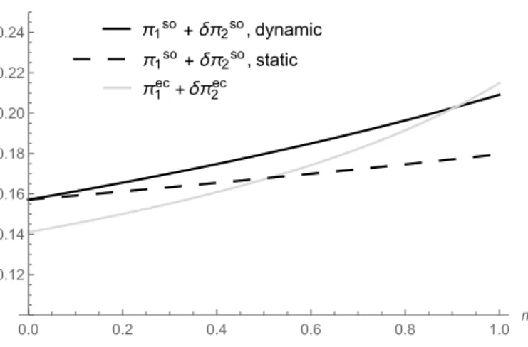
Figure 1 further illustrates Propositions 2 and 3 by plotting profits as a function of the market
size.25 It depicts (i) the maximum profits the firm can earn, given a period-1 sellout, under static
pricing, (ii) and under dynamic pricing; and (iii) the maximum profits the firm can earn, given
excess period-1 capacity (i.e. baseline profits). The superscript so stands for sellout, and the
superscriptec stands forexcess capacity. I normalize all profits by dividing bym, both in Figure 1 and in the figures that follow. Doing so helps with the exposition but has no effect on the ranking
of profits between (i), (ii), and (iii).
π1so+δπ2so, dynamic
π1ec+δπ2ec π1so+δπ2so, static
0.0 0.2 0.4 0.6 0.8 1.0 m
0.12 0.14 0.16 0.18 0.20 0.22 0.24
π/m
Figure 1: Profits as a function of market size
Figure 1 shows that even under static pricing, the firm finds it profitable to sell out and mislead
consumers for a wide variety of market sizes, m/0.51. The ability to engage in dynamic pricing
23
Other possible reasons for introductory pricing include compensating consumers who buy before they learn their true valuation (M¨oller and Watanabe 2010; Nocke et al. 2011), or exploiting network effects, for example by helping a firm establish its base before a rival (Katz and Shapiro, 1986).
24The same logic would apply if the firm could increase its capacity over time at a cost, although this would
reduce the size of the price discount and premium. If the firm could costlessly increase capacity, then it would set p1 =p2=A/2 and sell out for all values of the market size. Allowing the firm to carry over any excess capacity in
period 1 to serve consumers in period 2 would have no impact on pricing or profits.
25
further expands the circumstances under which selling out is optimal, to m / 0.91. Moreover, under dynamic pricing, there is a unique market size below which it is optimal to sell out, and
above which it is optimal to have excess capacity, just as under static pricing.26
π1so π1ec
0.0 0.2 0.4 0.6 0.8 1.0 m 0.07 0.08 0.09 0.10 π1/m (a)
π2so π2ec
0.0 0.2 0.4 0.6 0.8 1.0 m
0.06 0.08 0.10 0.12 0.14 0.16 0.18 0.20
π2/m
(b)
p1so p2so pec
0.0 0.2 0.4 0.6 0.8 1.0 m
0.16 0.18 0.20 0.22 0.24 0.26 0.28 0.30 p (c)
d1ec d2ec Kso=d
1so=d2so
0.0 0.2 0.4 0.6 0.8 1.0 m
0.1 0.2 0.3 0.4 0.5 d (d)
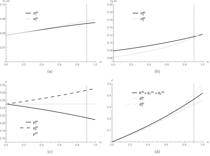
Figure 2: Per-period profits, prices, and capacity, as a function of market size
Figure 2 presents normalized per-period profits, optimal prices, and optimal capacity, under
dynamic pricing, given the same assumptions as in Figure 1. The vertical dashed line in each panel
gives the critical market size mu0.91. Panel (a) shows that sellouts always lead to lower
period-1 profits than having excess capacity. Sellouts give higher period-2 profits, as depicted in Panel
(b), except when the market is so large that the cost of not increasing sales over time outweighs
26
Proposition 3 does not specify that such a unique market size must always exist under dynamic pricing. However, simulations carried out for a wide range of parameter values, with m drawn fromU(0,1), all show such a unique value, m1 =m2. I have also shown analytically thatm1 = m2 always holds if m is drawn from U(0,1) and all
the benefit from misleading consumers. Panel (c) shows that the size of the period-1 discount
and the period-2 premium associated with sellouts is increasing in market size. Finally, Panel (d)
shows that the optimal capacity when selling out is often higher than demand in the baseline.
The implication is that firms may sometimes want to sell out not by restricting capacity, but by
combining a reasonably high capacity with a sufficiently low price.
I assume for the rest of the analysis that the firm can engage in dynamic pricing. In line with
Figure 2, the following result shows that the size of the period-1 discount and the period-2 premium
are increasing in the market size. It also demonstrates how the discount and premium depend on
the importance of the social payoff.
Proposition 4. Consider dynamic pricing, and suppose that m ∈ [0, m1), so that sellouts occur
in both periods. Then the period-1 price is decreasing in the market size and the importance of the
social payoff, whereas the period-2 price is increasing in these parameters, whenever the fraction
of uninformed consumers is sufficiently large: there exists α¯ ∈ (0,1) such that ∂p1
∂m < 0, ∂p1
∂λ < 0, ∂p2
∂m > 0, ∂p2
∂λ > 0 for all α ∈ ( ¯α,1]. Both prices are decreasing in the discount factor: ∂p1
∂δ < 0, ∂p2
∂δ <0 for all α ∈ (0,1]. Moreover, the ex-ante probability of selling out in both periods, P(q1 =
q2 =K), is increasing inδ and bounded below by F(m0)>0.
Both the period-1 discount and the period-2 premium will tend to be large if the social payoff
is important, as the firm then particularly benefits from misleading consumers. The proof of
Proposition 4 shows more generally that the derivative of the period-1 and period-2 price have
opposite sign, whether the derivative is taken with respect to m, λ, or α. It follows that a large period-1 discount should often precede a large period-2 premium.
An increase in the discount factor will instead result in a higher period-1 discount but a lower
period-2 premium. This result also reflects the firm’s intertemporal tradeoff when setting capacity.
The optimal capacity is increasing in the discount factor, because demand increases following a
sellout, and high capacity allows the firm to better take advantage of period-2 demand. Specifically,
high capacity means that the firm must offer a large period-1 discount in order to sell out, but can
serve all period-2 demand at close to the unconstrained optimal price, p=A/2.
costs in period 1 but benefits in period 2. Proposition 4 also shows that the probability of selling out
in both periods remains strictly positive even as the discount factor, the importance of the social
payoff, or the fraction of uninformed consumers tend to zero. In particular, the firm will always
mislead consumers in situations where they would react negatively to learning the true market size.
To explore how the firm’s strategic use of sellouts affects consumer welfare, I now compare
expected payoffs, from an ex ante perspective, in Proposition 3 to those from the baseline in
Proposition 1. Both intrinsic and social payoffs are included in the welfare calculations.
Proposition 5. Consider expected payoffs from Proposition 3. Then compared to expected payoffs
in the baseline:
(i) The firm earns higher expected profits.
(ii) All informed period-1 consumers and some uninformed period-1 consumers earn a higher
expected payoff, but at least some period-2 consumers earn a strictly lower expected payoff.
(iii) Ifδ is sufficiently large, then all informed period-2 consumers and some uninformed period-2 consumers earn a higher expected payoff.
Equilibrium profits can be no lower than baseline profits, since the firm can always follow its
baseline strategy. It can in fact do better still by setting price and capacity according to Proposition
3. Period-1 consumers then benefit from the period-1 discount, which makes buying cheaper and
also leads others to buy, generating a higher social payoff.
Period-2 consumers instead face a price premium following a sellout and may overestimate
demand. Some are misled into buying and are left worse off. However, the fact that they are misled
benefits others by increasing the social payoff from buying. When the discount factor is large,
the price premium is small, and its negative impact on consumers is dominated by the benefits of
bandwagon behavior. All informed consumers are then better off than in the baseline, as are all
uninformed consumers who would still have bought had they not been misled.
Formally, the statement of Proposition 4 allows δ to take on arbitrarily large values, including those greater than one. Such a high discount factor can be interpreted as the cumulative weight
that in each periodt= 1,2, . . . , T, a measuremof consumers enter the market, observe all previous prices and sales, decide whether to buy, and then exit. The equilibrium outcome of this new game
is identical to the one analyzed here, except the period-2 market outcome is repeated in all later
periods, and the firm has PT t=2δt
−1 as an effective discount factor.27 A large value of T and a
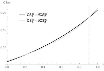
value of δ close to 1 in this new game would then correspond to δ1 in the two-period model. To address whether the strategic use of sellouts benefits consumers as a whole, Figure 3 plots
consumer surplus, divided by m, as a function of the market size, under the same assumptions as Figure 1. The proximity of both curves suggests that the overall impact of sellouts is quite small,
but this hides substantial heterogeneity across different consumer groups. Further simulations
suggest selling out will increase the surplus of both informed and uninformed consumers in period
1, compared to the baseline, but decrease that of both groups in period 2.
CS1so+δCS 2 so
CS1ec+δCS 2 ec
0.0 0.2 0.4 0.6 0.8 1.0 m
0.10 0.15 0.20
CS/m
Figure 3: Consumer surplus as a function of market size
Figure 3 also shows that consumers as a whole benefit from sellouts if the market is neither
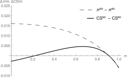
too large nor too small. To see this more clearly, Figure 4 plots the vertical difference between the
curves in Figure 3, so the gain in surplus per consumer that arises from sellouts, as a function of
the market size. Consistent with Figure 3, the dark curve in Figure 4 lies below the horizontal axis
27
for small and large values ofm but above it for intermediate values.28
CSso -CSec πso-πec
0.2 0.4 0.6 0.8 1.0 m
-0.010
-0.005
0.005 0.010 0.015 0.020 0.025 Δπ/m,ΔCS/m
Figure 4: Gain in surplus and profits from sellouts as a function of market size
The impact of strategic sellouts on consumer surplus can be divided into three effects. First,
sellouts generate increased variability in pricing, compared to the baseline, which reduces consumer
surplus. The period-2 premium dissuades consumers from buying precisely when demand is high
and buying would yield a high social payoff. Second, sellouts mislead some uninformed period-2
consumers into buying, which reduces consumer surplus. Third, misleading some consumers into
buying increases the social payoff of other buyers, which increases consumer surplus.
When the market is very large, the first effect (variability in pricing) dominates, and sellouts
leave consumers worse off. The second and third effects are small because consumers do not
sustantially overestimate demand following a sellout, so that being misled does little to change
behavior. When the market is very small, sellouts again leave consumers worse off, but now because
the second effect (misleading consumers into buying) dominates. The first effect is small because
sellouts have little impact on pricing, as illustrated in Figure 2, and so is the third effect, since a
low market size implies a low social payoff regardless of consumer beliefs. Figure 4 shows that the
third effect (increasing the social payoff) can dominate for a relatively large range of intermediate
market size, so that sellouts lead to higher consumer surplus than in the baseline.
Figure 4 also shows that the firm’s interests are often broadly aligned with those of consumers, in
28
terms of when sellouts leave them better off. For many values of the market size where sellouts lead
to higher consumer surplus, they also leads to higher firm profits. This is the case approximately
for all m ∈ [0.22,0.91]. Interests are also broadly aligned when the market is sufficiently large, approximately for all m ∈ (0.91,1], as both consumers and the firm then benefit from excess capacity. As a result, equilibrium expected consumer surplus is higher than in the baseline, precisely
because the firm can mislead consumers. The same applies to total surplus, which exceeds that in
the baseline for almost all realizations of the market size.
5
Robustness
I now discuss the extent to which modifying certain assumptions might affect the results described
in Section 4.
Consumers care about demand rather than quantity sold. Instead of assuming that
consumers’ willingness to pay is directly increasing in their beliefs about demand, an alternative
would be to assume that willingness to pay was directly increasing in beliefs about sales. This
assumption would effectively mean that consumers were not conformists, but that the product
exhibited network effect. Demand may differ from sales if the firm is capacity constrained, so a
natural question is whether the firm would still strategically use sellouts to mislead consumers.
With network effects, a period-1 sellout would still lead consumers to overestimate period-2
demand, and potentially increase their expected network payoff from buying. A difference compared
with Section 4 is that restricting capacity would reduce this expected payoff by limiting sales. In
particular, a capacity constraint would reduce the willingness to pay of period-1 consumers, who
would reason that some of them might not be served. Period-2 consumers who observe a sellout
would become more optimistic about demand, but may worry that high demand cannot translate
into high sales. This would likely push the firm to set a higher price when restricting capacity, and
also reduce the firm’s incentive to sell out.
Capacity is a strategic choice. The firm’s optimal strategy as described in Section 4 consists
when it is large. These results would change if capacity was exogenous. Sellouts would no longer
occur when the market was very small, relative to capacity, either because there would be too few
consumers to sell out, or because selling out would require too large of a price discount. Sellouts
would instead occur when the market was very large, simply because the firm could not serve all
these consumers at its preferred price.
That being said, consumer inference following a sellout would remain unchanged, and the firm
would still benefit from selling out as long as capacity was not too high. Specifically, suppose the
firm would face a small amount of excess capacity if it charged the baseline price, given the realized
market size. Then it would have an incentive to offer a small price discount so as to sell out and
mislead consumers. It could then take advantage of the resulting increase in demand by charging
a subsequent price premium.
Price commitment. The firm’s optimal strategy does not depend on whether it can ex ante
commit to a period-2 price, because this price has no impact on the willingness to pay of period-1
consumers. These consumers cannot buy at the period-2 price since they no longer remain in the
market. Their social payoff from buying is also independent of the period-2 price, since it depends
only on demand from consumers in their own cohort.
Price commitment could matter if period-1 consumers were willing and able to strategically delay
their purchases. The firm might then want to commit to a higher period-2 price to discourage delay.
Regarding incentives to delay, consumers could learn from observing the period-1 market outcome,
but Propositions 2 and 3 suggest that they could also face a price increase (under dynamic pricing)
or possible rationing (under static pricing). Whether consumers would have an incentive to delay
would depend on how they evaluate this tradeoff, in particular given their partial sophistication.29
Price commitment would also matter if the social payoff for period-1 consumers depended in
part on period-2 demand. The firm would then benefit from committing to a low period-2 price,
which would increase the willingness to pay of consumers in period 1 by increasing their social
payoff. However, the overall features of the analysis would remain unchanged. Given the period-1
market outcome, consumers’ willingness to pay in period 2 would still be increasing in beliefs about
29
the market size, and the firm could still use sellouts to mislead these consumers.
Firm uncertainty about demand. The assumption that the firm knows the exact period-1
demand can be relaxed, for example by adding a small amount of noise. Doing so will not change
the main qualitative conclusions from Section 4 but will change two specific results: that period-1
sellouts can sometime occur for reasons unrelated to misleading consumers, i.e. in the baseline, and
that sellouts under dynamic pricing are never accompanied by strictly positive excess demand.
Proposition 6. Consider dynamic pricing, and let be an unobserved random variable with mean zero that follows an atomless distribution with full support on [−∆,∆]. Suppose that period-1
demand is D1 = d1(p1, F1) +, and period 2 demand is D2 =d2(p2, F2), with dt(pt, Ft) given by
(13) for t∈ {1,2}. Then:
(i) The probability of a period-1 sellout in the baseline, where D1 is revealed after period 1, is
zero: P(q1 =K) = 0.
(ii) Consider any m ∈[0, m1), for which Proposition 3 shows that the firm sells out in period
1: d1(p1, F) =K. In the limit as ∆ tend to zero, the probability of strictly positive excess demand
tends to one : lim∆→0P(D1 > K) = 1.
If the firm is uncertain about period-1 demand, then its only concern in the baseline is to
serve as many consumers as possible, so the optimal capacity is almost surely higher than period-1
demand. The situation changes when consumers cannot directly observe demand, because they
then form very different beliefs when demand is slightly below capacity than when it is slightly
above. The firm is willing to accept a high probability of a small amount of excess demand to
ensure that it sells out, so it can reap the benefits in the following period. This logic applies more
broadly to situations where the firm is uncertain about demand but still knows more than certain
consumers. If the firm could not mislead consumers, then demand uncertainty would lead it to
increase capacity, to serve all demand in both periods. If instead the firm can mislead consumers
6
Conclusion
This paper helps provide a rationale as to why firms may point to past sellouts to promote
fu-ture sales, in settings where conformist consumers care about product popularity. Specifically, it
explores how observing a sellout may favorably influence consumer beliefs about demand and
en-courage bandwagon behavior. Consistent with evidence on limited strategic reasoning, I assume
that consumers neglect how the firm’s actions may reflect its private information when updating
their beliefs, which raises the possibility that they may be mislead. Sellouts allow the firm to do
just that, to mislead consumers into believing demand is higher than it truly is, by effectively
withholding unfavorable information. This possibility to mislead consumers provides the firm with
incentives to sell out when demand is low and can lead to introductory pricing. Sellouts hurt some
consumers but help others, and can lead to higher overall consumer surplus.
Appendix
Proof of Lemma 1. Assume for now that pt,dit, and dut take on values such that (8) and (9) imply
θit∈(−(1−A), A) and θtu∈(−(1−A), A). Rearrange (10) to obtain
dit=
(1−α)m 1−(1−α)λm
(A+λdut −pt), (16)
and substitute into (11) to give
dut =αm
A+λ
Z 1
0
dutdFt+λ Z 1
0
(1−α)m0 1−(1−α)λm0
(A+λdut −pt)
dFt−pt
. (17)
Define X(Ft) ≡ dut/(αm(A−pt)), which is independent of m, since θut is independent of m, and
sincedu
t =αm(A−θut). Write
Substituting (18) into (16) yields
dit= ((1−α)m(A−pt))
1 +αmλX(Ft)
1−(1−α)λm
. (19)
Substituting (18) into (17) and solving forX(Ft) gives (12), so
X(Ft)≡
1 +R01
(1−α)λm0 1−(1−α)λm0
dFt(m0)
1−αλR01m0dFt(m0)−αλ R1
0
(1−α)λm02
1−(1−α)λm0
dFt(m0)
.
If pt∈[0, A), then (18), (19), and (12), together with λ <1−A and m≤1, imply 0< dut +dit<
m≤1. Looking at (8) and (9), and again using λ < 1−A, confirms that θit∈(−(1−A), A) and θut ∈(−(1−A), A), so demand is uniquely determined by (18), (19), and (12). If instead pt≥A,
then demand is uniquely determined bydit=dut = 0.
Proof of Lemma 2. Let f denote the pdf of F, and ft the pdf of Ft, for t ∈ {1,2}. Bayes’ rule
implies
f1(m|K, p1) = P
(K, p1|m)
P(K, p1)
f(m), (20)
withP(K, p1) = R1
0 P(K, p1|m
0)dF(m0), where
P(K, p1|m) follows from the firm’s equilibrium
strat-egy. Consumers update beliefs according to Bayes’ rule, except they use P(K, p1|m) = P(K, p1).
Substituting into (20) yieldsf1(m|K, p1) =f(m), or equivalently F1(m|K, p1) =F(m), confirming
that period-1 beliefs are given by the prior.
For period 2, Bayes’ rule implies
f2(m|K, p1, q1, p2) = P
(q1, p2|m, K, p1)
P(q1, p2|K, p1)
f1(m|K, p1)
=
P(q1|m, K, p1)P(p2|m, K, p1, q1)
P(q1|K, p1)P(p2|K, p1, q1)
f1(m|K, p1),
(21)
withP(p2|K, p1, q1) = R1
0 P(p2|m
0, K, p
1, q1)dF(m0), whereP(p2|m, K, p1, q1) follows from the firm’s
P(p2|K, p1, q1). Together withf1(m|K, p1) =f(m), this implies
f2(m|K, p1, q1, p2) = P
(q1|m, K, p1)
P(q1|K, p1)
f(m),
where integrating gives the distribution function
F2(m|K, p1, q1, p2) = Rm
0 P(q1|m
0, K, p
1)dF(m0) R1
0 P(q1|m0, K, p1)dF(m0)
, (22)
withR01P(q1|m0, K, p1)dF(m0) =P(q1|K, p1). The probabilityP(q1|m, K, p1) follows from consumer
equilibrium strategies and the firm’s choice ofK andp1. Specifically, demand d1(p1, F) is given by
(13), with sales q1 =min{d1, K}.
From (13),d1is strictly increasing inm, for anyp1 < A. Hence, for anyp1< Aand resultingd1,
there is a unique market sizem(d1, p1) consistent with this demand and price, which is increasing
ind1. The right-hand side of (13) is strictly decreasing inp1, som(d1, p1) is strictly increasing in
p1.
If d1 < K, then consumers observe q1 = min{d1, K} < K, and they infer d1 = q1. This
implies P(q1|m0, K, p1) = 1 for m0 = m(d1, p1) and P(q1|m0, K, p1) = 0 for all m0 6= m(d1, p1),
wherem(d1, p1) =m, the true market size. Expression (22) then reduces to Fm, given by (14), as
required.
If d1 ≥ K, then consumers observe q1 = min{d1, K} = K, and they infer d1 ≥ K. This
implies P(q1|m0, K, p1) = 1 for all m0 ≥ m(K, p1) and P(q1|m0, K, p1) = 0 for all m0 < m(K, p1).
Expression (22) then reduces to Fm(K,p1)+, given by (15), as required. The threshold m(K, p1)
is strictly increasing in p1 and K, since m(d1, p1) is strictly increasing in both arguments. When
K =d1, the threshold reduces tom(d1, p1) =m, the true market size.
Proof of Proposition 1. Supposed1 is revealed after period 1. By the proof of Lemma 2, period-2
beliefs are then F2 = Fm, which are independent of K, p1, and q1. Demand is d2(p2, Fm), which
by (13) is proportional to (A−p2). Hence, period-2 profits, π2 =p2d2(p2, Fm), are proportional
period-2 price of p2 = A/2, provided that K ≥ d2(A/2, Fm). Period-2 profits are therefore π2 =
d2(A/2, Fm)A/2 if K ≥ d2(A/2, Fm), and π2 < d2(A/2, Fm)A/2 if K < d2(A/2, Fm). They are
independent ofp1.
Period-1 demand isd1(p1, F), which by (13) is proportional to (A−p1). Hence, period-1 profits,
π1 = p1d1(p1, F), are proportional to p1(A−p1), provided that K ≥d1(p1, F). Taking the
first-order condition implies an optimal period-1 price of p1 = A/2, provided that K ≥ d1(A/2, F).
Period-1 profits are therefore π1 = d1(A/2, F)A/2 if K ≥ d1(A/2, F) and π1 < d1(A/2, F)A/2 if
K < d1(A/2, F). Hence, the firm maximizes its objective function (2) by setting p1 = p2 =A/2,
with K ≥ max{d1(A/2, F), d2(A/2, Fm)}. The firm can only sell out in both periods if m =m0,
where m0 is the unique value of m for which d1(p, F) = d2(p, Fm). The probability that m =m0
equals zero, since the market size is drawn from an atomless distribution.
Proof of Proposition 2. Let πso denote the maximum profits the firm can earn given price and capacity that yield a period-1 sellout. Let πec denote the maximum profits it can earn given price and capacity that yield excess period-1 capacity. Specifically, by (2), F1 =F and Lemma 2, write
πec = max
K,p1,p2
(min{d1(p1, F), K}p1+δmin{d2(p2, Fm), K}p2) s.t. d1(p1, F)< K, (23)
πso = max
K,p1,p2
min{d1(p1, F), K}p1+δmin{d2(p2, Fm(K,p1)+), K}p2
s.t. d1(p1, F)≥K, (24)
where static pricing gives the additional constraintp1 =p2 ≡p.
Demand in (23) is identical to that in the baseline, so Proposition 1 implies
πec= A
2(d1(A/2, F) +δd2(A/2, Fm)), (25)
which the firm earns by setting p=A/2, with K≥max{d1(A/2, F), d2(A/2, Fm)}.
From (24), write πso=p(K+δmin{d
2(p, F2), K}), where F2 =Fm(K,p)+. Ifd1(p, F)> K and
d1(p2, F2)> K, thenπso =pK(1 +δ). Deviating top+, for >0 but small, then yields strictly
higher profits, π= (p+)K(1 +δ)> πso, sod1(p, F)> K and d1(p2, F2)> K cannot be optimal.
K +, for > 0 but small, yields profits π = p(K ++δmin{d2(p, Fm(K+,p)+), K +}). To establishπ > πso, I now show thatd2(p, Fm(K+,p)+)> d2(p, Fm(K,p)+). Notice first that Lemma 2
implies m(K, p)< m(K+, p). Setting Ft=Fm(K,p)+ in (12) gives
X(Fm(K,p)+)≡
1 +R1 0
(1−α)λm0 1−(1−α)λm0
dFm(K,p)+(m0) 1−αλR1
0 m0dFm(K,p)+(m0)−αλ R1
0
(1−α)λm02
1−(1−α)λm0
dFm(K,p)+(m0).
The expression in each integral is positive and increasing in m0, and (15) implies Fm(K+,p)+ ≤ Fm(K,p)+ for all m0 ∈ [0,1], with Fm(K+,p)+ < Fm(K,p)+ for all m(K, p) < m0 < 1. Thus,
X(Fm(K+,p)+)> X(Fm(K,p)+), so that (13) impliesd2(p, Fm(K+,p)+)> d2(p, Fm(K,p1)+). It follows
that d1(p, F) > K and d1(p, F2) ≤ K cannot be optimal. Hence, to earn πso, the firm must set
price and capacity such that d1(p, F) =K, where Lemma 2 then impliesF2 =Fm+.
Write πso = p(K+δmin{d2(p, Fm+), K}), with d1(p, F) = K. The above argument, to
es-tablish d2(p, Fm(K+,p)+) > d2(p, Fm(K,p1)+), showed that d2(p, Fm(K,p)+) is increasing in m(K, p).
Moreover, by (15), beliefs Fm(K,p)+ are identical to the priorF if and only if m(K, p) = 0. Thus,
(13) implies d2(p, Fm(K,p)+) ≥d1(p, F) for all m(K, p)∈[0,1]. It follows that profits can be
writ-ten as πso = pd1(p, F)(1 +δ). Expression (13) shows that d1(p, F) is proportional to (A−p),
so the firm maximizes profits when selling out by setting p = A/2, and K = d1(p, F), to earn
πso= A2d1(A/2, F)(1 +δ).
Comparingπso = A2d1(A/2, F)(1 +δ) withπec = A2(d1(A/2, F) +δd2(A/2, Fm) yieldsπso ≥πec
if and only if d1(A/2, F) ≥ d2(A/2, Fm). Recall that m0 ∈ (0,1) is defined as the value of m
satisfying X(Fm) =X(F), and that X(Fm) = 1/(1−λm) is strictly increasing in m. Thus, from
(13), it follows that πso≥πec if and only ifm≤m0.
Proof of Proposition 3. Consider (23) and (24) from the proof of Proposition 2, where once again,
demand in (23) is identical to that in the baseline. This implies that πec is given by (25), which the firm earns by settingp1 =p2 =A/2, withK ≥max{d1(A/2, F), d2(A/2, Fm)}.
Write πso = Kp1 +δmin{d2(p2, F2), K}p2, where F2 = Fm(K,p1)+. If d2(p2, F2) > K, then
πso = Kp1 +δKp2. Deviating to p2+, for > 0 but small, then yields strictly higher profits,
K and d1(p1, F) > K, then πso = Kp1+δd2(p2, Fm(K,p1)+)p2. Deviating to p1 +, for > 0
but small, yields π = K(p1 +) +δmin{d2(p2, Fm(K,p1+)+), K}p2. To establish π > π
so, it
is sufficient to show that d2(p2, Fm(K,p1+)+) > d2(p2, Fm(K,p1)+). Notice that Lemma 2 implies
m(K, p1) < m(K, p1+). Thus, the same argument as in the proof of Proposition 2 that showed
X(Fm(K+,p)+)> X(Fm(K,p)+), also impliesX(Fm(K,p1+)+)> X(Fm(K,p1)+). Combined with (13), this yields d2(p2, Fm(K,p1+)+)> d2(p2, Fm(K,p1)+). It follows that the firm sets d1(p1, F) =K.
Hence, profits from selling out areπso=d
1(p1, F)p1+δd2(p2, Fm+)p2, whered1(p1, F) =K and
d2(p2, Fm+)≤K. I now show thatd2(p2, Fm+) =K. Suppose instead thatd2(p2, Fm+)< K. Then
by (13), the firm must set p2 =A/2, to maximize period-2 profits, d2(p2, Fm+)p2. The inequality
d1(p1, F)> d2(A/2, Fm+) then impliesp1 < A/2. This is becaused(p, F)< d(p, Fm+) for allm >0,
by F =F0+ from (15), and by ∂m∂ d(p, Fm+). Moreover, p1 < A/2 implies ∂p∂1d1(p1, F)p1 >0, by
(13). Write πso = d1(p1, F)p1+δd2(A/2, Fm+)(A2), where K = d1(p1, F). Now suppose the firm
deviates to period-1 price p1+ and capacity d1(p1+, F)> d2(A/2, Fm+), for >0 but small.
This deviation yields π =d1(p1+, F)(p1+) +δd2(A/2, Fm+)(A2)> πso, by ∂p∂1d1(p1, F)p1 >0.
It follows that the firm will setd1(p1, F) =d2(p2, Fm+) =K, so that
πso=d1(p1, F)p1+δd2(p2, Fm+)p2 s.t. d1(p1, F) =d2(p2, Fm+) =K, (26)
evaluated at the optimalK. To solve for this optimal capacity, and by extension the corresponding prices, define
C(F)≡ d1(p1, F) A−p1
=
αX(F) + (1−α) 1−(1−α)λm
m, (27)
C(Fm+)≡
d2(p2, Fm+)
A−p2
=
αX(Fm+) + (1−α)
1−(1−α)λm
m, (28)
using (13), which are independent of price. Substituting (27) and (28) into (26) gives
πso=K
A− K C(F)
+δK
A− K C(Fm+)