Flexible margin-based classification techniques

(1)

Flexible Margin-Based Classiﬁcation Techniques

Seo Young Park

A dissertation submitted to the faculty of the University of North Carolina at Chapel Hill in partial fulﬁllment of the requirements for the degree of Doctor of Philosophy in the Department of Statistics and Operations Research.

Chapel Hill 2010

Approved by

Advisor: Dr. Yufeng Liu Reader: Dr. Douglas G. Kelly Reader: Dr. J. S. Marron Reader: Dr. Wei Sun

(2)

c

⃝ 2010

(3)

ABSTRACT

SEO YOUNG PARK: Flexible Margin-Based Classiﬁcation Techniques (Under the direction of Dr. Yufeng Liu)

Classification is a very useful statistical tool for information extraction. Among numerous classification methods, margin-based classification techniques have attracted a lot of attention. It can be typically expressed as a general minimization problem in the form of 𝑙𝑜𝑠𝑠+𝑝𝑒𝑛𝑎𝑙𝑡𝑦, where the loss function controls goodness of fit of the training data and the penalty term enforces smoothness of the model. Since the loss function decides how functional margins affect the resulting margin-based classifier, one can modify the existing loss functions to obtain classifiers with desirable properties.

(4)

ACKNOWLEDGEMENTS

I owe my deepest gratitude to my advisor, Professor Yufeng Liu, whose guidance, encouragement, and support enabled me to enjoy my research and complete my dissertation work successfully. He helped me explore the subject with his keen insight and immense knowledge, and provided many opportunities for various kinds of collaborative research. Beyond and above his obligations as a thesis advisor, he has been an integral if not essential advocate to any and all of my potential future pursuits. I could not imagine having a better advisor for my Ph.D. study.

I wish to express my sincere appreciation to committee members, Douglas G. Kelly, J. Steve Marron, Wei Sun, Hao Helen Zhang for their valuable comments and suggestions on this dissertation.

(5)

List of Figures

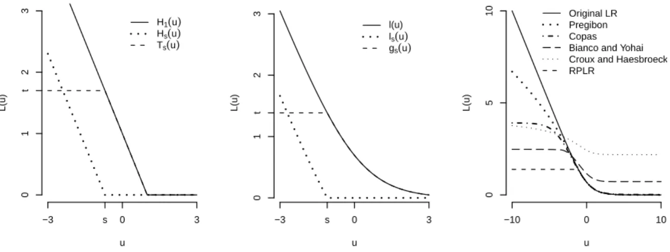
1.1 Plot of diﬀerent loss functions. . . 3 2.1 Left: Plot of the functions𝐻₁(𝑢),𝐻_𝑠(𝑢), and𝑇_𝑠(𝑢) with𝐻_𝑠(𝑢) = [𝐻₁(𝑢)−𝐻₁(𝑠)]₊

and 𝑇𝑠(𝑢) =𝐻1(𝑢)−𝐻𝑠(𝑢); Middle: Plot of the functions𝑙(𝑢), 𝑙𝑠(𝑢), and 𝑔𝑠(𝑢)

with 𝑙𝑠(𝑢) = [𝑙(𝑢)−𝑙(𝑠)]+ and 𝑔𝑠(𝑢) = 𝑙(𝑢)−𝑙𝑠(𝑢) ; Right: Plot of the loss

functions of the original logistic regression, Pregibon’s resistant fitting model, Copas’ misclassification model, and the RPLR. . . 10 2.2 Illustration plot of the effect of outliers with an outlier far away from its own

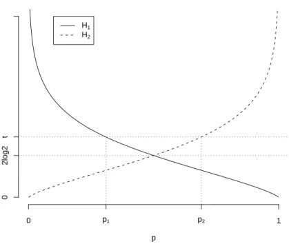
class. The RPLR boundary is much robust than that of the original PLR. . . 11 2.3 Plot of 𝐻1 and 𝐻2 for Theorem 2 in Section 2.4.3. The condition 𝑡 > 𝐻1(𝜋, 𝑝)

and 𝑡 > 𝐻2(𝜋, 𝑝) hold only when 𝑝∈[𝑝1, 𝑝2]. . . 18

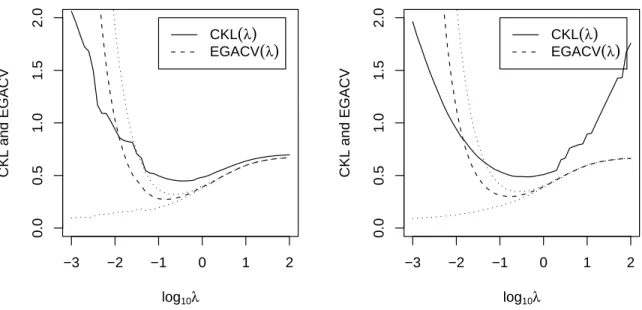
2.4 Left: An illustration plot of𝐶𝐾𝐿(𝜆) and𝐸𝐺𝐴𝐶𝑉(𝜆) from the example in Section 2.6; Right: Average curves of𝐶𝐾𝐿(𝜆) and 𝐸𝐺𝐴𝐶𝑉(𝜆) based on 100 replications. 28 2.5 Plot of typical training sets for Example 2.7.1.1 (the left panel) and Example

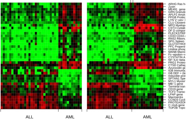
2.7.2.2 (the right panel) as well as the corresponding decision boundaries. . . 31 2.6 Heat maps of the Leukaemia data in Section 2.7.2.1. The left panel is for the

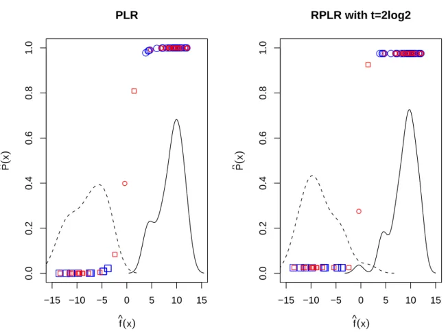
training set and the right panel is for the testing set. The red and green colors represent high and low expression values respectively. . . 33 2.7 Plot of the estimated class probabilities against the estimated values of the linear

predictor 𝑓(𝒙) = 𝒘𝑇_𝒙₊_𝑏 _{for the PLR and the RPLR with} _𝑡 _{= 2 log 2. The}

solid and the dashed lines are the estimated density curves of the values of linear predictor for ALL and AML class, respectively. . . 34 2.8 Biplot on PCA of the lung cancer data in Section 2.7.2.2. . . 36 3.1 Plot of loss function𝑔(𝑢) with diﬀerent values of𝑣 . . . 43 3.2 Illustration of the eﬀect of 𝛼𝑖𝑦𝑖 in the standard SVM. The left and right panel

illustrates that a positive and negative 𝛼𝑖𝑦𝑖 tends to push the boundary towards

to the left and right side, respectively. . . 46 3.3 Plots of the eﬀect of diﬀerent values of 𝑣 on the BSVM. . . 47 3.4 A graphical illustration of the robustness of the BSVM: the decision boundary of

the BSVM stays stable when there is an extreme outlier, while that of the SVM moves dramatically towards the outlier. . . 48 3.5 A graphical comparison of the SVM vs. BSVM: the decision boundary of the

(9)

3.6 Plots of the asymptotic variances in (3.15). . . 54 3.7 Left: Illustration of the data set in Example 3.6.1.1. Right: Illustration of the

path of 𝒘with respect to 𝑣 in Example 3.6.1.1. . . 60 3.8 Plot of several BCM loss functions indexed by 𝑎. . . 64 4.1 Plot of the 0−1 loss function and the composite squared loss functions with

𝛾 = 0,0.5,1. . . 83 4.2 Scatter plots of typical datasets of Example 4.5.1, 4.5.2, and 4.5.3. . . 88 4.3 Left: Plot of the average test errors of the multicategory CLS classiﬁer based on

100 replications with 𝛾 = 0.0,0.1,0.2,⋅ ⋅ ⋅ ,1.0 for Example 4.5.1.1. Right: Plot of the average probability estimation errors of the multicategory CLS classiﬁer based on 100 replications with𝛾 = 0.0,0.5, and 1.0 for Example 4.5.1.1. . . 90 4.4 Left: Plot of the average test errors of the multicategory CLS classiﬁer based

on 100 replications with 𝛾 = 0.0,0.1,0.2,⋅ ⋅ ⋅ ,1.0 for Example 4.5.1.2. Here, the results with ’tuned𝛾’ are the results when𝛾is tuned among{0,0.5,1}along with

𝜆. Right: Plot of the average probability estimation errors of the multicategory CLS classiﬁer based on 100 replications with 𝛾 = 0.0,0.5, and 1.0 for Example 4.5.1.2. . . 92 4.5 Left: Plot of the average test errors of the multicategory CLS classiﬁer based on

100 replications with 𝛾 = 0.0,0.1,0.2,⋅ ⋅ ⋅ ,1.0 for Example 4.5.1.3. Right: Plot of the average probability estimation errors of the multicategory CLS classiﬁer based on 100 replications with𝛾 = 0.0,0.5, and 1.0 for Example 4.5.1.3. . . 94 4.6 Plot of the estimated class probabilities for subjects in the testing set of the

Leukemia data. The heights of cyan, bright yellow, and dark green bars stand for the estimated probability of ALLB, ALLT, and AML, respectively. . . 96 4.7 Heat maps of the Leukemia data. The left panel is for the training set and the

(10)

List of Tables

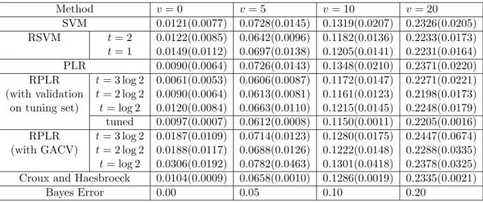
2.1 Testing errors of the simulated linear example (Example 2.7.1.1) . . . 32

2.2 Class probability estimation errors of the simulated linear example (Example 2.7.1.1) . . . 35

2.3 Testing errors of the simulated nonlinear example (Example 2.7.1.2) . . . 36

2.4 Class probability estimation errors of the simulated nonlinear example (Example 2.7.1.2) . . . 36

2.5 Testing errors of the Lung Cancer Data example in Section 7.2.2. . . 37

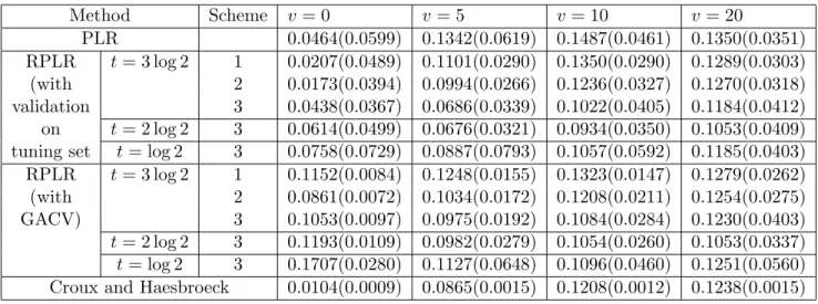
3.1 Testing errors of the simulated linear example (Example 3.6.1.1) . . . 61

3.2 Testing errors of the simulated nonlinear example (Example 3.6.1.2) . . . 62

3.3 Testing errors of the lung cancer data example in Section 3.6.2. . . 62

4.1 Estimated Test errors based on 100 replications for Example 4.5.1.1. The rows with tuned 1 and tuned 2 show the results when𝜆is tuned at the same time with𝛾 among {0,0.1,0.2,⋅ ⋅ ⋅,1.0}, and among {0,0.5,1}, respectively. The Bayes error is 0.2043. . . 89

4.2 Estimated Test errors based on 100 replications for Example 4.5.1.2. The rows with tuned 1 and tuned 2 show the results when𝜆is tuned at the same time with𝛾 among {0,0.1,0.2,⋅ ⋅ ⋅,1.0}, and among {0,0.5,1}, respectively. The Bayes error is 0.0459 and 0.1538 when 𝜎= 0.5 and 𝜎= 0.7, respectively. . . 91

(11)

Chapter 1 Introduction

1.1 Background on Classiﬁcation

Classification, as an example of supervised learning, is a procedure that builds a model based on a training dataset to predict the class memberships for new examples with only covariates available. It can be understood as a special form of regression with the response variable being categorical. If the response variable is binary, that is, there are only two classes, it is known as binary classification. If there are more than two classes, we have multicategory classification.

For simplicity, we first focus on binary classification, and multicategory classification will be discussed in Chapter 4. In binary classification, we want to build a classifier based on a training sample {(𝒙𝑖, 𝑦𝑖)}𝑖=1,⋅⋅⋅,𝑛, where 𝒙𝑖 ∈ R𝑑 is a 𝑑-dimensional vector of predictors, and 𝑦𝑖 ∈ {+1,−1} is its class label. Typically it is assumed that the training data are distributed

according to an unknown probability distribution 𝑃(𝒙, 𝑦). Binary classification is to find a decision rule 𝜙(⋅) and predict the class membership as ˆ𝑦 =𝜙(𝒙) for any future observation 𝒙. One important goal is to minimize the misclassification rate𝑃(𝑌 ∕=𝜙(𝑿)).

(12)

the value of 𝑓(𝒙) close to zero indicates that 𝑥 is near the decision boundary. Thus, high value of 𝑦𝑓(𝒙) implies the classification for𝒙is correct with much confidence, and as the value of 𝑦𝑓(𝒙) goes to negative infinity, it means the classification was wrong with high confidence, which is not desirable. Hence, we can say that functional margin 𝑦𝑓(𝒙) shows ‘correctness’ of the classification, and we generally want values of functional margin to be high.

To make use of the functional margin, one can think of ﬁnding the decision function 𝑓(𝒙) by minimizing the sum of values of a certain loss function in 𝑦𝑓(𝒙). That is, minimizing ∑_𝑛

𝑖=1𝐿(𝑦𝑖𝑓(𝒙𝑖)), where 𝐿(𝑢) is a loss function, can be a criterion to find a decision function 𝑓(𝒙). One of the natural loss functions is the 0−1 loss function,𝐿(𝑦𝑓(𝒙)) =𝐼(𝑦𝑓(𝒙)⩽0), which is hard to implement computationally. Hence, it is often to use convex surrogate loss functions in practice. However, this formulation often provides poor classification rules of𝑓(𝒙), because of potential overfitting. A common solution to this is to add a constraint on the parameters to stabilize or toshrinkthe estimates. Then margin-based classifiers can be summarized using the regularization framework in the following form

min

𝑓∈ℱ

𝑛

∑

𝑖=1

𝐿(𝑦_𝑖𝑓(𝒙_𝑖)) +𝜆𝐽(𝑓), (1.1)

whereℱis the decision function class of interest, and𝐿(𝑢) is the loss function which is a function of the margin𝑦𝑓(𝒙),𝐽(𝑓) is the penalty term that controls the smoothness of the model, and𝜆

is a tuning parameter which balances the tradeoﬀ between those two. In some practice, one may also use min𝑓∈ℱ𝐶

∑_𝑛

𝑖=1𝐿(𝑦𝑖𝑓(𝒙𝑖)) +𝐽(𝑓) instead, but it is equivalent to (1.1) since𝜆plays the

same role as 1/𝐶. The loss function controls goodness of ﬁt of the model, and the penalization term helps avoid overﬁtting so that good generalization can be obtained.

In the literature, there exist a number of margin-based classifiers. Using different loss func-tions, we can formulate different classifiers such as the Support Vector Machine (SVM) (Vapnik, 1998; Cristianini and Shawe-Taylor, 2000), the Penalized Logistic Regression (PLR) (Wahba, 1999; Lin et al., 2000), Distance-Weighted Discrimination (DWD) (Marron et al., 2007) and so on. Due to the definition of the functional margin, many well-known margin-based methods use nonincreasing loss functions on𝑦𝑓(𝑥) which encourages large functional margin.

(13)

u

l(u)

−2 −1 0 1 2 3 4

0

1

2

3

0−1 loss

Hinge loss (SVM) Logistic loss

Exponential loss (AdaBoost)

Figure 1.1: Plot of diﬀerent loss functions.

modify the loss function to obtain different classifiers with desirable properties. One important contribution of this research is to study various modifications of the loss function to derive several classifiers with different properties.

Next we briefly overview several commonly used margin-based classifiers including the PLR, the SVM, and Boosting. Each of them can be understood as a special form of (1.1) with a different loss function 𝐿(𝑢). The loss functions of these classifiers are plotted in Figure 1.1 for graphical comparison.

1.2 Several Existing Methods

1.2.1 Penalized Logistic Regression

In the standard logistic regression model for binary classiﬁcation, one assumes the logit, the log odds ratio, can be modeled as a linear function in covariates. Speciﬁcally, the model can be written as follows:

log𝑃(𝑌 = +1∣𝑿)

𝑃(𝑌 =−1∣𝑿) =𝒘

(14)

where𝑿 and𝑌 denote the vector of explanatory variables and the class label, respectively. The coeﬃcients of logistic regression (𝒘, 𝑏) can be estimated by the method of Maximum Likelihood (ML) (McCullagh and Nelder, 1989). Once the ML estimators for (1.2) are obtained, the sign of𝑓(𝒙), where𝑓(𝒙) =𝒘𝑇_𝒙₊_𝑏_{can be used as the class membership estimates. This is because}

the model (1.2) implies that𝑃(𝑌 = +1∣𝑿=𝒙)>0.5 if𝑓(𝒙)>0, and𝑃(𝑌 = +1∣𝑿=𝒙)⩽0.5 otherwise.

The linear logistic regression can be generalized to the PLR by adding a constraint on the parameters. In particular, le Cessie and van Houwelingen (1992) proposed PLR, which maximizes the log-likelihood subject to a constraint on the 𝐿2 norm of the coeﬃcients. Wahba

(1999) showed the linear PLR is equivalent to ﬁnding𝑏and𝒘which solves (1.1) whereℱ ={𝑓 :

𝑓(𝒙) =𝒘𝑇_𝒙₊_𝑏_}_,_𝐿₍_𝑢_{) =}_𝑙₍_𝑢_{) = log (1 +}_𝑒−𝑢_),_𝐽₍_𝑓_{) =} 1

2∥𝒘∥22, and𝜆 >0 is a tuning parameter.

For a nonlinear problem, theory of reproducing kernel Hilbert spaces can be applied and then the kernel PLR has ℱ ={𝑓 :𝑓(𝒙) =𝑟(𝒙) +𝑏, 𝑟(𝒙) ∈ ℋ𝐾} and 𝐽(𝑓) =∥𝑟∥ℋ𝐾, where𝑟(𝒙) =

∑_𝑛

𝑖=1𝑣𝑖𝐾(𝒙𝑖,𝒙) and 𝐾 is the kernel function (Wahba, 1999). Properties of the reproducing

kernel and the representative theorem imply that∥𝑟∥2_ℋ_𝐾 =𝒗𝑇_𝑲𝒗 _where_𝒗 _{= (}_𝑣

1, . . . , 𝑣𝑛)𝑇 and

𝑲is an𝑛×𝑛positive deﬁnite matrix with its𝑖1𝑖2-th element𝐾(𝒙𝑖1,𝒙𝑖2) (Kimeldorf and Wahba,

1971).

1.2.2 Support Vector Machine

The Support Vector Machine (SVM) can be viewed as a member of the regularization framework (1.1). It employs the hinge loss function𝐿(𝑦𝑓(𝒙)) = [1−𝑦𝑓(𝒙)]+. (See Figure 1.1.) The value

of 𝐿(𝑦𝑓(𝒙)) increases as𝑦𝑓(𝒙) becomes smaller and it stays at zero when 𝑦𝑓(𝒙) ⩾1. That is, the SVM puts positive loss on the misclassified data points but 0 loss on the correctly classified observations once 𝑦𝑓(𝒙) becomes greater than 1. Hence the data points with 𝑦𝑓(𝒙) ⩾ 1 have no influence on the SVM solution. To explain further, we rewrite the SVM optimization in the following primal problem with the penalty term𝐽(𝑓) = 1₂∥𝒘∥2 for the standard SVM,

min

(𝑏,𝒘)

1 2∥𝒘∥

2₊_𝐶 𝑛

∑

𝑖=1

(15)

To handle the hinge loss, we introduce𝑛nonnegative slack variables,𝜉_𝑖, 𝑖= 1,⋅ ⋅ ⋅, 𝑛. Then (1.3) is equivalent to

min

(𝑏,𝒘)

1 2∥𝒘∥

2₊_𝐶 𝑛

∑

𝑖=1 𝜉𝑖

subject to 𝜉_𝑖⩾1−𝑦_𝑖𝑓(𝒙_𝑖);𝜉_𝑖⩾0,∀𝑖= 1,⋅ ⋅ ⋅ , 𝑛.

We can transform this problem into its corresponding dual problem with the Lagrange mul-tipliers𝛾𝑖 and 𝛼𝑖,𝑖= 1,⋅ ⋅ ⋅, 𝑛, for contraints. The Lagrange primal function is

𝔏(𝒘, 𝑏,𝜶) = 1

2∥𝒘∥

2₊_𝐶∑𝑛 𝑖=1

𝜉_𝑖+

𝑛

∑

𝑖=1

𝛼_𝑖[1−𝑦_𝑖𝑓(𝒙_𝑖)−𝜉_𝑖]− 𝑛

∑

𝑖=1

𝛾_𝑖𝜉_𝑖 (1.4)

where𝐶= 1/𝜆, and𝛼𝑖 ⩾0 and𝛾𝑖 ⩾0 are the Lagrange multipliers. Setting derivatives to zero,

we have

∂𝔏

∂𝒘 = 𝒘−

𝑛

∑

𝑖=1

𝑦𝑖𝛼𝑖𝒙𝑖=0 (1.5)

∂𝔏

∂𝑏 = −

𝑛

∑

𝑖=1

𝑦𝑖𝛼𝑖 = 0 (1.6)

∂𝔏

∂𝜉𝑖 = 𝐶−𝛼𝑖−𝛾𝑖= 0, (1.7)

with Karush-Kuhn-Tucker (KKT) conditions of the convex optimization theory

𝛼𝑖(1−𝑦𝑖𝑓(𝒙𝑖)−𝜉𝑖) = 0 (1.8)

𝛾𝑖𝜉𝑖= 0. (1.9)

Substituting (1.5)-(1.9) into (1.4) gives the dual problem of the SVM

min

𝜶

1 2

𝑛

∑

𝑖,𝑗=1

𝑦_𝑖𝑦_𝑗𝛼_𝑖𝛼_𝑗⟨𝒙_𝑖,𝒙_𝑗⟩ − 𝑛

∑

𝑖=1 𝛼_𝑖

subject to

𝑛

∑

𝑖=1

𝑦𝑖𝛼𝑖= 0; 0⩽𝛼𝑖 ⩽𝐶,∀𝑖= 1,⋅ ⋅ ⋅, 𝑛. (1.10)

Using the𝛼𝑖 obtained from (1.10),𝒘 can be calculated as

∑_𝑛

(16)

by (1.7). Thus the decision boundary becomes 𝑓(𝒙) =∑𝑛_𝑖=1𝛼_𝑖𝑦_𝑖⟨𝒙_𝑖,𝒙⟩+𝑏. Because of (1.8), we can see that𝛼_𝑖 >0 implies𝑦_𝑖𝑓(𝒙_𝑖)⩽1 and actually that is the only case that (𝒙_𝑖, 𝑦_𝑖) aﬀects the solution. On the other hand, when 𝛼𝑖 = 0, the observation (𝒙𝑖, 𝑦𝑖) has no impact on the

solution. We call 𝒙𝑖 with 𝛼𝑖 >0 a Support Vector (SV), which is the observation misclassiﬁed

or correctly classiﬁed but with less conﬁdence, satisfying𝑦𝑖𝑓(𝒙𝑖)⩽1.

1.2.3 Boosting

Boosting has been a very important machine learning method in the past 20 years. The original boosting algorithm, AdaBoost (Freund and Schapire, 1997), is an iterative procedure that com-bines many weak classifiers updating weights of training observations. In particular, initially a weak classifier is trained on the training data with all equal weights. Then, for each iteration, the weights of the misclassified observations are increased and the weak classifier is recalculated based on the newly weighted data. Then a score is assigned to the classifier based on the mis-classification rate. After repeating this procedure for sufficiently many times, the final classifier is defined as weighted sum of all the classifiers from the iterations with the scores as weights.

Friedman et al. (2000) showed that the AdaBoost is approximating to ﬁtting additive model using the exponential loss function. Thus, we can view the AdaBoost as a special member of regularization problem in (1.1) with loss𝐿(𝑦𝑓(𝒙)) = exp(−𝑦𝑓(𝒙)). (See Figure 1.1.)

1.3 Outline

In the following chapters, we propose several new margin-based classiﬁers with various loss functions.

∙ In Chapter 2, we introduce the Robust Penalized Logistic Regression (RPLR) and study its properties. Moreover, we derive a computational algorithm as well as methods for class probability estimation and tuning parameter selection. Numerical demonstration includes simulated examples and the application on Lung Cancer Dataset.

(17)

their properties, asymptotic behaviors, and the entire solution path for eﬃcient computa-tion. Numerical results include the simulated example and the Lung Cancer Data.

∙ In Chapter 4, we discuss multicategory classiﬁers and propose the multicategory Composite Least Squares (CLS) classiﬁer. In addition, its properties, procedure for class probability estimation, and a computational algorithm are derived. Numerical results are included.

(18)

Chapter 2 Truncation for robustness

2.1 Introduction

The PLR is a commonly used classification method in practice. It is a generalization of the standard logistic regression with a penalty term on the coefficients. Similar to the SVM, the PLR can be fit in the regularization framework with 𝑙𝑜𝑠𝑠+𝑝𝑒𝑛𝑎𝑙𝑡𝑦 (Wahba, 1999; Lin et al., 2000). The loss function controls goodness of fit of the model, and the penalization term helps avoid overfitting so that good generalization can be obtained.

For the standard SVM, its hinge loss function is unbounded, as a result, the SVM classifier can be sensitive to outliers (Shen et al., 2003; Liu and Shen, 2006). Wu and Liu (2007) proposed the Robust SVM (RSVM) as a modification of the original SVM by truncating the hinge loss function. They showed that through the operation of truncation, the impact of outliers can be reduced, consequently, the resulting classifier may be more robust.

Comparing to the SVM, the PLR uses the logistic loss which is also unbounded. Therefore, similar to the SVM, the PLR can be sensitive to extreme outliers as well. In this chapter, we propose the Robust Penalized Logistic Regression (RPLR), which uses truncated logistic loss function. Because truncation reduces the impact of misclassiﬁed outliers, the RPLR is more robust and accurate than the standard PLR. Comparisons of the proposed RPLR with the existing robust logistic regression methods are discussed as well.

(19)

the PLR, one can use the estimated classification function, i.e. the estimated logit function, to derive the corresponding probability estimate. When we replace the logisitic loss by its truncated version, properties of the corresponding classification function may not preserve all class probability information any more. To solve this problem, we propose three different schemes for class probability estimation. Properties and performance of these three schemes are explored as well.

Although the original logistic loss function is convex, its truncated version becomes non-convex. Consequently, the corresponding minimization problem involves difficult non-convex optimization. To implement the RPLR, we decompose the non-convex truncated logistic loss function into the difference of two convex functions. Then, using this decomposition, we apply the difference convex (d.c.) algorithm to obtain the solution of the RPLR through iterative convex minimization.

The tuning parameter plays an important role in the RPLR implementation. To select a good tuning parameter, we develop the Estimated Generalized Approximate Cross Validation (EGACV) procedure and compare its performance with the cross validation method.

In the following sections, we describe the new proposed method in more details with theo-retical justiﬁcation and numerical examples. Section 2.2 reviews the PLR and gives a maximum likelihood interpretation. In Section 2.3 we review some related robust logistic regression meth-ods in the literature. In Section 2.4 we describe the RPLR and explore its theoretical properties. The methods for class probability estimation are also introduced. Section 2.5 develops the d.c. algorithm to solve the nonconvex minimization problem for the RPLR. In Section 2.6 we explore various ways to select the tuning parameter. Numerical results are presented in Section 2.7 and Section 2.8 provides some discussions. The proofs of theorems are included in Section 2.9.

2.2 Penalized Logistic Regression

As mentioned in Section 1.2.1, the PLR solves (1.1) with the logistic loss function 𝑙(𝑢) = log(1 +𝑒−𝑢_{). Here, we brieﬂy review the PLR and its likelihood interpretation.}

Notice that the loss function 𝑙(𝑢) = log(1 +𝑒−𝑢_{) is a smooth decreasing function as shown}

(20)

u

L(u)

−3 s 0 3

0

1

t

2

3

H1(u) Hs(u) Ts(u)

u

L(u)

−3 s 0 3

0

1

t

2

3

l(u) ls(u) gs(u)

u

L(u)

−10 0 10

0

5

10 Original LR Pregibon Copas Bianco and Yohai Croux and Haesbroeck RPLR

Figure 2.1: Left: Plot of the functions𝐻₁(𝑢),𝐻_𝑠(𝑢), and𝑇_𝑠(𝑢) with𝐻_𝑠(𝑢) = [𝐻₁(𝑢)−𝐻₁(𝑠)]₊ and 𝑇𝑠(𝑢) =𝐻1(𝑢)−𝐻𝑠(𝑢); Middle: Plot of the functions 𝑙(𝑢), 𝑙𝑠(𝑢), and 𝑔𝑠(𝑢) with 𝑙𝑠(𝑢) =

[𝑙(𝑢)−𝑙(𝑠)]+ and 𝑔𝑠(𝑢) =𝑙(𝑢)−𝑙𝑠(𝑢) ; Right: Plot of the loss functions of the original logistic

regression, Pregibon’s resistant ﬁtting model, Copas’ misclassiﬁcation model, and the RPLR.

infinity. This causes high impact of outliers with very small (negative) value of 𝑦_𝑖𝑓(𝒙_𝑖). As a result, the coefficient estimates of the PLR can be affected by outliers far from their own classes. To further illustrate the effect of outliers on the PLR, we randomly generate 2-dimensional separable data and apply the PLR to obtain a classification boundary. As shown in the left panel of Figure 2.2, the PLR works very well without outliers. However, if we randomly select one of the observations and move it away from its own class, then the classification boundary of the PLR is pulled towards to that outlier, as shown in the right panel of Figure 2.2. As a result, the corresponding misclassification rate will become higher. In contrast, our new proposed method is much more robust to the outlier so that its classification boundary is more accurate. The effect of outliers on the PLR can also be interpreted using maximum likelihood. The likelihood function of unpenalized logistic regression can be written as

ℒ(𝑏,𝒘) =

𝑛

∏

𝑖=1 𝑃(𝒙𝑖)

1+_𝑦𝑖

2 (1−𝑃(𝒙_𝑖)) 1−_𝑦𝑖

2 , (2.1)

where𝑃(𝒙) =𝑃(𝑌 = +1∣𝑿 =𝒙). Then, we can plug in the logit function (1.2) into (2.1), and the corresponding maximizer of ℒ(𝑏,𝒘) is the solution of the logistic regression. Note that the

(21)

−4 −3 −2 −1 0 1 2

−2

−1

0

1

2

3

4

x1 x2

Bayes PLR RPLR

−4 −3 −2 −1 0 1 2

−2

−1

0

1

2

3

4

x1 x2

Bayes PLR RPLR

Figure 2.2: Illustration plot of the eﬀect of outliers with an outlier far away from its own class. The RPLR boundary is much robust than that of the original PLR.

Therefore to maximize the likelihood, one needs to ﬁnd (𝒘, 𝑏) to make 𝑃(𝒙𝑖) big when 𝑦𝑖 = 1

and small when𝑦𝑖 =−1. However, this could be sensitive to outliers. To illustrate this further,

assume there is one data point 𝑥𝑖 with 𝑦𝑖 = +1 which locates far from the other data points

of class +1 but closer to data of class −1 as illustrated in the right panel of Figure 2.2. Using the solution (𝒘, 𝑏) without the outlier, the corresponding 𝑃(𝒙𝑖) for the outlier will be very

small because𝒙𝑖 is closer to the data of class −1. Consequently, the ML method would select

(𝒘, 𝑏) which will make𝑃(𝒙𝑖) larger to obtain bigger likelihood at the expense of other entries’

classiﬁcation accuracy. This results in the boundary moving towards to the outlier. In the next section, we discuss some literature on robust logistic regression.

2.3 Literature on Robust Logistic Regression

(22)

Welsch, 1982; Morgenthaler, 1992). Stefanski et al. (1986) and K¨unsch et al. (1989) modiﬁed original score function of the logistic regression to obtain bounded sensitivity, which is a concept introduced by Krasker and Welsch (1982). Morgenthaler (1992) used 𝐿1-norm instead of 𝐿2

-norm in the likelihood, resulting in a weighted score function of the original score function. Cantoni and Ronchetti (2001) focused on robustness of inference rather than the model.

Pregibon (1982) suggested resistant ﬁtting methods which taper the standard likelihood to reduce the inﬂuence of extreme observations. In particular, he proposed to estimate (𝒘, 𝑏) by solving

min

𝑓∈ℱ

𝑛

∑

𝑖=1 ℎ(𝒙𝑖)𝜌

(

𝑑_𝑖 ℎ(𝒙𝑖)

)

, (2.2)

where𝜌(𝑢) is a tapering function,ℎ(𝒙) is a factor which controls leverage of each observation, and 𝑑𝑖 is negative log likelihood, that is, 𝑑𝑖 = −

[

1+𝑌𝑖

2 log𝑃(𝒙𝑖) +1−2𝑌𝑖log(1−𝑃(𝒙𝑖))

] . Note that this reduces to standard maximum likelihood estimation of the logistic regression when

ℎ(𝒙) ≡ 1 and 𝜌(𝑢) = 𝑢. The particular tapering function Pregibon (1982) proposed to use is the Huber’s loss function

𝜌(𝑢) = ⎧  ⎨

 ⎩

𝑢 if𝑢⩽𝐻,

2(𝑢𝐻)1/2−𝐻 otherwise,

(2.3)

where 𝐻 is a prespeciﬁed constant. In order to compare with our new method, we provide a new view of the method by Pregibon (1982) in the loss function framework. In particular, with

𝜌 in (2.3) andℎ(𝒙)≡1, we can reduce (2.2) to

min

𝑓∈ℱ

𝑛

∑

𝑖=1

𝑙Pregibon(𝑦𝑖𝑓(𝒙𝑖)),

where

𝑙Pregibon(𝑢) =𝜌(𝑙(𝑢)) = ⎧  ⎨

 ⎩

log (1 +𝑒−𝑢₎ _if_𝑢_⩾₋_{log (}_𝑒𝐻₋₁₎

2(𝐻log (1 +𝑒−𝑢₎₎1/2₋_𝐻 _otherwise. (2.4)

(23)

Figure 2.1 for comparison. As shown in the plot,𝑙Pregibon(𝑢) grows as𝑢goes to negative inﬁnity, but less rapidly than the loss function of the original logistic regression𝑙(𝑢). Consequently, the resulting coeﬃcient estimates become less sensitive to extreme observations. However, the value of𝑙Pregibon(𝑢) remains to be unbounded, hence the impact of outliers can still be large.

Bianco and Yohai (1996) proposed a consistent and more robust version of Pregibon’s esti-mator, by adding a bias correction term. More speciﬁcally, they suggested to solve

min

𝑓∈ℱ

𝑛

∑

𝑖=1

𝜌(𝑑𝑖) +𝐶𝑖, (2.5)

with the 𝑑𝑖 previously deﬁned and the bias correction term𝐶𝑖, where 𝐶𝑖 = 𝐺(𝑃(𝒙𝑖)) +𝐺(1− 𝑃(𝒙𝑖))−𝐺(1), 𝐺(𝑡) =

∫_𝑡

0 𝜌′(−log𝑢)𝑑𝑢, and

𝜌(𝑡) = ⎧  ⎨

 ⎩

𝑡−_2𝑐𝑡2 if𝑡⩽𝑐 𝑐

2 otherwise,

(2.6)

where 𝑐 is a constant. Croux and Haesbroeck (2003) pointed out that the minimizer of (2.5) with𝜌(𝑡) in (2.6) does not exist quite often, in particular, the minimizer tends to be inﬁnity. To overcome this problem, they suggested to use

𝜌(𝑡) = ⎧  ⎨

 ⎩

𝑡e−√𝑑 _if_𝑡_⩽_𝑑

−2e−√𝑡_{(1 +}√_𝑡_{) + e}−√𝑑_{(2(1 +}√_𝑑_{) +}_𝑑_{) otherwise,} (2.7)

and

𝐺(𝑡) = ⎧  ⎨

 ⎩

𝑡e−√−log𝑡_{+ e}1/4√_𝜋_Φ(√₂₍1 2+

√

−log𝑡))−e1/4√_𝜋 _if_𝑡_⩽_𝑑

e−√𝑑_𝑡₋_e−1/4√_𝜋_{+ e}1/4√_𝜋_Φ(√₂₍1 2 +

√

𝑑)) otherwise,

(2.8)

where𝑑is a constant and Φ is the normal cumulative distribution function. To view the method by Croux and Haesbroeck (2003) in the loss function framework, we show that the problem (2.5) with𝜌(𝑡) in (2.7) is equivalent to solving

min

𝑓∈ℱ

𝑛

∑

𝑖=1

(24)

where

𝑙CH(𝑢) = 𝐼_{_𝑢_⩾₋_log(e𝑑₋₁₎_}

[

log(1 + e−𝑢)e−√𝑑+ e−√𝑑_1+e1−𝑢 −e−1/4

√

𝜋+ e1/4√𝜋Φ(√2(1₂ +√𝑑)) ]

+𝐼_{_𝑢<₋_log(e𝑑₋₁₎_}

[

−2e−√log(1+e−𝑢₎

(1 +√log(1 + e−𝑢_{)) + e}−√𝑑_{(2(1 +}√_𝑑_{) +}_𝑑₎ 1

1+e−𝑢e−

√

log(1+e−𝑢₎

+ e1/4√_𝜋_Φ(√₂₍1 2+

√

log(1 + e−𝑢₎₎₎₋_e−1/4√_𝜋]

+𝐼_{_𝑢_⩾_log(e𝑑₋₁₎_}

[

1 1+e𝑢e−

√

log(1+e𝑢₎

+ e1/4√𝜋Φ(√2(1₂+√log(1 + e𝑢₎₎₎₋_e−1/4√_𝜋]

+𝐼_{_𝑢<log(e𝑑₋₁₎_}

[

e−√𝑑 1

1+e𝑢 −e−1/4

√

𝜋+ e1/4√_𝜋_Φ(√₂₍1 2 + √ 𝑑)) ] . (2.10) The loss function (2.10) is plotted in the right panel of Figure 2.1.

Another attempt to achieve robustness was made by Copas (1988), who modeled contamina-tion of class labels in the training data. Speciﬁcally, it is assumed that the class label𝑦∈ {1,−1}

was transposed with a small probability𝛾. As a result, the response𝑦can be 1 with probability

𝑃∗(𝒙), where

𝑃∗(𝒙) = (1−𝛾)𝑃(𝒙) +𝛾(1−𝑃(𝒙)). (2.11)

Using (1.2) and (2.11), the log-likelihood with𝑃∗_{(𝒙) becomes}

𝑛

∑

𝑖=1

[ 1 +𝑌𝑖

2 log𝑃

∗_(𝒙

𝑖) +1−₂𝑌𝑖 log(1−𝑃∗(𝒙𝑖))

] = 𝑛 ∑ 𝑖=1 [ 1 +𝑌_𝑖

2 log

1 +𝛾(𝑒−𝑓(𝒙𝑖)−1) 1 +𝑒−𝑓(𝒙𝑖) +

1−𝑌_𝑖

2 log

1 +𝛾(𝑒𝑓(𝒙𝑖)−1) 1 +𝑒𝑓(𝒙𝑖)

] = 𝑛 ∑ 𝑖=1 [

𝐼_(𝑌_𝑖₌₁₎log1 +𝛾(𝑒−𝑌𝑖𝑓(𝒙𝑖)−1)

1 +𝑒−𝑌𝑖𝑓(𝒙𝑖) +𝐼(𝑌𝑖=−1)log

1 +𝛾(𝑒−𝑌𝑖𝑓(𝒙𝑖)−1) 1 +𝑒−𝑌𝑖𝑓(𝒙𝑖)

]

=

𝑛

∑

𝑖=1

log1 +𝛾(𝑒−𝑌𝑖𝑓(𝒙𝑖)−1) 1 +𝑒−𝑌𝑖𝑓(𝒙𝑖) .

(2.12)

To view this in the loss framework, we get the equivalent problem of log likelihood maximization in (2.12) as follows

min

𝑓∈ℱ

𝑛

∑

𝑖=1

𝑙Copas(𝑦𝑖𝑓(𝒙𝑖)), (2.13)

where 𝑙Copas(𝑢) = log 1+𝑒−𝑢

(25)

reduces the inﬂuence of outliers by truncating the logistic loss function.

2.4 Robust Penalized Logistic Regression

2.4.1 Truncated Loss for Robustness

Although most of the previous methods done on robust logistic regression takes the likelihood point of view, it can be transformed into the loss function framework as shown in the previous section. In this thesis, we take a diﬀerent approach to achieve robustness for the logistic regres-sion. In particular, we develop a new classiﬁer by truncating the loss function directly rather than modifying the log likelihood function.

Due to the unboundedness of the logistic loss function, it assigns large loss values for points far from their own classes. Consequently, the resulting classifiers will be affected by those outliers. To reduce the effect of outliers, we propose a novel Robust version of the PLR (RPLR), which truncates the loss function of the PLR. Specifically, we propose to use the truncated logistic loss function𝑔𝑠(𝑢) = min(𝑙(𝑢), 𝑙(𝑠)) instead of𝑙(𝑢). Here𝑠⩽0 represents the location of truncation.

As illustrated in the middle panel of Figure 2.1,𝑔𝑠(𝑦𝑓(𝒙)) increases as𝑦𝑓(𝒙) decreases, but once 𝑦𝑓(𝒙) becomes less than𝑠,𝑔𝑠(𝑦𝑓(𝒙)) becomes a constant. This implies that 𝑔𝑠 becomes bigger

as an observation gets further away from the classiﬁcation boundary up to an upperbound. For outliers located further away from the boundary satisfying𝑦𝑓(𝒙)⩽𝑠, the loss stays at a constant

𝑙(𝑠) so that the outliers cannot further influence the classification boundary. This is in contrast to the untruncated version whose impact grows to infinity. Also, it differs from the other existing methods we covered in the previous section in the sense that the effect of extreme observations stays the same once 𝑦𝑓(𝒙) becomes less than 𝑠, while that of others keeps increasing. Note that 𝑠 determines the level of truncation. When 𝑠= −∞, no truncation occurs, thus the loss is the same as the original logistic loss. As 𝑠 gets closer to 0, we have more truncation on the loss which may reduce the effect of outliers further. Therefore, 𝑔𝑠(𝑢) contains a group of loss

functions indexed by 𝑠.

(26)

[𝐻₁(𝑢)−𝐻₁(𝑠)]₊. As shown in the left panel of the Figure 2.1, the truncated hinge loss function

𝑇_𝑠(𝑦𝑓(𝒙)) stays the same once 𝑦𝑓(𝒙) becomes less than 𝑠, similarly to 𝑔_𝑠(𝑦𝑓(𝒙)). But once

𝑦𝑓(𝒙) becomes greater than 1, the loss function of the RSVM𝑇𝑠(𝑦𝑓(𝒙)) becomes 0. In contrast,

the loss function of the RPLR 𝑔𝑠(𝑦𝑓(𝒙)) remains small but positive. That is, the RSVM does

not use the information about data points with 𝑦𝑓(𝒙) >1, while the RPLR uses all the data points to build a classification boundary. This can be beneficial for the RPLR as reflected in the simulation results in Section 2.7 .

From the likelihood point of view, minimizing ∑𝑛_𝑖=1𝑔𝑠(𝑦𝑖𝑓(𝒙𝑖)) is equivalent to maximizing

𝑛

∏

𝑖=1

𝑄+(𝒙𝑖)

1+_𝑦𝑖

2 (1−𝑄−(𝒙_𝑖)) 1−_𝑦𝑖

2 , (2.14)

where 𝑄+_{(𝒙) = max(}_𝑃_(𝒙)_, 1

1+𝑒−𝑠) and 𝑄−(𝒙) = min(𝑃(𝒙),_1+𝑒1𝑠). Interestingly, (2.14) has a similar form as that of the logistic regression in (2.1). The diﬀerence is that the 𝑖-th factor is

𝑄+_(𝒙

𝑖) or 1−𝑄−(𝒙𝑖), instead of 𝑃(𝒙𝑖) and 1−𝑃(𝒙𝑖), depending on 𝑦𝑖. Hence, maximizing

(2.14) is equivalent to ﬁnding (𝒘, 𝑏) which gives big 𝑄+_{(𝒙) when} _𝑦 _{= +1 and small} _𝑄−_(𝒙)

when𝑦=−1. By deﬁnition,𝑄+_{(𝒙) can not get extremely small because it is lower bounded by}

(1 +𝑒−𝑠₎−1_{. Similarly,} _𝑄−_{(𝒙) can not get extremely big. Therefore outliers may not inﬂuence}

(2.14) as much comparing to (2.1). As a result, the maximizer of (2.14) can be less sensitive to outliers. For the toy example illustrated in Figure 2.2, the classiﬁcation boundary of the original PLR deteriorates dramatically when there exists an extreme outlier in the dataset. In contrast, the RPLR boundary is very stable whether there is an outlier or not.

2.4.2 Fisher Consistency

(27)

we consider three diﬀerent truncation locations 𝑠= 0,−log 3, and −log 7 for the RPLR. The corresponding values of the logistic loss are 𝑙(0), 2𝑙(0), and 3𝑙(0), respectively. Our numerical results suggest that𝑠=−log 3 with 𝑙(𝑠) = 2𝑙(0) gives the best performance. This matches the Fisher consistency results for multicategory classiﬁcation.

So far, we have focused on the standard case, i.e., treating different types of misclassification equally. Sometimes, it can be natural to impose different costs for different types of misclassifi-cation. For example, it can be more severe to misclassify an observation of class +1 to class−1 than that of class −1 to +1. Then it is sensible to put a bigger cost for the first kind of mis-classification than the second type. Lin et al. (2002) discussed the weighted SVM to deal with nonstandard situations such as different misclassification costs for different classes. Recently, Wang et al. (2007) applied weighted learning to large margin classifiers for probability estima-tion. In addition to Fisher consistency of non-weighted robust logistic regression, we investigate similar properties of the weighted robust logistic regression.

Let (1−𝜋, 𝜋) with 0< 𝜋 <1 be the weights for class +1 and class−1 respectively, then the weighted version of the RPLR becomes

min

𝑓∈ℱ(1−𝜋)

∑

𝑦𝑖=1

𝑔𝑠(𝑦𝑖𝑓(𝒙𝑖)) +𝜋

∑

𝑦𝑖=−1

𝑔𝑠(𝑦𝑖𝑓(𝒙𝑖)) + 𝜆₂𝐽(𝑓), (2.15)

where𝜆 >0 balances the goodness of ﬁt, measured by the loss function, and the smoothness of𝑓. If 𝜆= 0, the objective function in (2.15) reduces to the unpenalized robust logistic regression. Note that the expectation of the weighted loss part in (2.15) is 𝐸[ℎ𝜋(𝑌)𝑔𝑠(𝑌 𝑓(𝑿))], where ℎ𝜋(1) = 1−𝜋 and ℎ𝜋(−1) =𝜋.

To understand the RPLR further, we need to explore the property of weighted robust logistic regression. The following theorem discusses the theoretical minimizer of the truncated logistic loss.

Theorem 1. The minimizer𝑓∗

𝜋 of 𝐸[ℎ𝜋(𝑌)𝑔𝑠(𝑌 𝑓(𝑿))] has the same sign as𝑃(𝒙)−𝜋.

Theorem 1 indicates that the sign of 𝑓∗

𝜋 is the same as sign(𝑃(𝒙) −𝜋). Thus, sign(𝑓𝜋∗)

provides a natural estimate of sign(𝑃(𝒙)−𝜋). In particular, if𝑓∗

𝜋 >0, then𝑃(𝒙)> 𝜋, otherwise 𝑃(𝒙) ⩽𝜋. This oﬀers a natural procedure for class probability estimation. In particular, one can estimate𝑓∗

(28)

p

0 p1 p2 1

0

2log2

t

H1 H2

Figure 2.3: Plot of𝐻1 and 𝐻2 for Theorem 2 in Section 2.4.3. The condition 𝑡 > 𝐻1(𝜋, 𝑝) and 𝑡 > 𝐻2(𝜋, 𝑝) hold only when𝑝∈[𝑝1, 𝑝2].

it can be used for class probability estimation, as discussed further in Section 2.4.3.

2.4.3 Probability Estimation

Lin (2002) showed that under certain conditions the solution ˆ𝑓𝜋 of (2.15) approaches 𝑓𝜋∗ =

argmin𝐸[ℎ𝜋(𝑌)𝑔𝑠(𝑌 𝑓(𝑿))]. Therefore, we can use the property of 𝑓𝜋∗ to design estimators of

class probabilities ˆ𝑃(𝒙). In the simplest scenario where 𝜋 = 1/2 and 𝑠 = −∞, we use the regular logistic loss and (2.15) reduces to the ordinary PLR. In that case, it is well known that the minimizer of𝐸[𝑙(𝑌 𝑓(𝑋))] is 𝑓 = log [𝑝(𝑋)/(1−𝑝(𝑋))]. Then a natural estimator of 𝑃(𝒙) is𝑒𝑓ˆ_/_{(1 +}_𝑒𝑓ˆ_).

When we use the truncated loss function, the minimizer of 𝐸[ℎ𝜋(𝑌)𝑔𝑠(𝑌 𝑓(𝑋))] does not

al-ways maintain enough information to obtain class probability estimation. The following theorem establishes the minimizer of𝐸[ℎ𝜋(𝑌)𝑔𝑠(𝑌 𝑓(𝑋))].

Theorem 2. Deﬁne 𝐻₁(𝜋, 𝑃(𝒙)) = log [1 + 1/𝜏(𝑃(𝒙), 𝜋)] + [1/𝜏(𝑃(𝒙), 𝜋)] log [1 +𝜏(𝑃(𝒙), 𝜋)],

(29)

Then, for 𝑡=𝑔_𝑠(𝑠),

𝑓_𝜋∗ = ⎧        ⎨

       ⎩

log𝜏(𝑃(𝒙), 𝜋) if 𝑡 > 𝐻1(𝜋, 𝑃(𝒙))and 𝑡 > 𝐻2(𝜋, 𝑃(𝒙))

−∞ if 𝑡 < 𝐻1(𝜋, 𝑃(𝒙))and 𝐻1(𝜋, 𝑃(𝒙))> 𝐻2(𝜋, 𝑃(𝒙)) ∞ if 𝑡 < 𝐻2(𝜋, 𝑃(𝒙))and 𝐻1(𝜋, 𝑃(𝒙))< 𝐻2(𝜋, 𝑃(𝒙)) −∞,∞ if 𝑡 < 𝐻₁(𝜋, 𝑃(𝒙)) =𝐻₂(𝜋, 𝑃(𝒙)).

Theorem 2 implies that we can use𝑓∗

𝜋to express class probability only when𝑓𝜋∗= log𝜏(𝑃(𝒙), 𝜋) =

log_𝜋(1(1−₋𝜋)𝑃_𝑃₍(_𝒙𝒙₎₎). Otherwise we cannot reconstruct𝑃(𝒙) using𝑓∗

𝜋. To further illustrate the

relation-ship between𝑓∗

𝜋 and𝑃(𝒙), we consider𝐻1 and 𝐻2 in the case that𝜋 = 1/2, which is plotted in

Figure 2.3. When𝑃(𝒙)∈[𝑝1, 𝑝2] with𝑡=𝐻1(𝜋, 𝑝1) and𝑡=𝐻2(𝜋, 𝑝2), then 𝑓𝜋∗ = log𝜋(1(1−−𝜋)𝑃𝑃((𝒙𝒙))).

However, when𝑃(𝒙)∈/ [𝑝1, 𝑝2], 𝑓𝜋∗ is either ∞or−∞, which does not have enough information

to recover𝑃(𝒙). For this reason, we need to explore other schemes to estimate𝑃(𝒙). To estimate the class probability, we propose the following three schemes.

Scheme 1 Since the RPLR works only for estimation of 𝑃(𝒙) ∈ [𝑝1, 𝑝2], we can consider

utilizing it for those𝑝, and using the ordinary PLR for𝑃(𝒙)∈/ [𝑝1, 𝑝2]. Notice that this scheme

is valid only for𝑡 >2 log 2, because if 𝑡⩽2 log 2,𝑝₁ =𝑝₂ and 𝑡 is smaller than 𝐻₁ and 𝐻₂ for any 𝑃(𝒙) as shown in Figure 2.3. Thus by Theorem 2, the RPLR does not work for estimation of any𝑃(𝒙) when 𝑡⩽2 log 2.

This scheme is a valid approach in the sense that estimation of𝑃(𝒙)∈[𝑝1, 𝑝2] is more critical

than that of𝑃(𝒙)∈/[𝑝1, 𝑝2]. Usually the data points with very small𝑃(𝒙) or very big𝑃(𝒙) are

easier to classify and we are more certain about the class membership of those points. However, class membership prediction for data points with 𝑃(𝒙) near 1/2 is not only diﬃcult, but also highly aﬀected by outliers. Thus estimation of the class probability becomes more important for those points. Therefore, we use the RPLR for estimation of 𝑃(𝒙) ∈ [𝑝1, 𝑝2], and use the

ordinary PLR for 𝑃(𝒙)∈/ [𝑝1, 𝑝2].

Scheme 2 The second scheme is motivated by the idea that we can shift𝑝₁and𝑝₂by changing

(30)

that this method is applicable only when 𝑡 > 2 log 2, and here we illustrate the case with

𝑡 = 3 log 2. More specifically, we use seven different 𝜋’s such as 𝜋₁ = 1/2, 𝜋₂ = 1/5, 𝜋₃ = 4/5, 𝜋4 = 1/20, 𝜋5 = 19/20, 𝜋6 = 1/91, 𝜋7 = 90/91, which give different estimable regions

for 𝑃(𝒙), [0.310,0.690], [0.105,0.358], [0.642,0.899], [0.024,0.101], [0.895,0.976], [0.005,0.024], [0.976,0.995]. Using ˆ𝑓𝑗 which denotes the solution from the RPLR with 𝜋𝑗, we can construct

the estimator ˆ𝑃𝑗_{(𝒙) =}_𝑒𝑓ˆ𝑗_/_{(1 +}_𝑒𝑓ˆ𝑗_);_𝑗 _{= 1}_,_{⋅ ⋅ ⋅} _,_{7, to estimate}_𝑃_{(𝒙) in the corresponding region.}

There are some drawbacks of the second scheme. First, there are overlaps between the estimable regions. Moreover, the RPLR with diﬀerent 𝜋’s can give contradictory inference about 𝑃(𝒙). To solve this, for given ˆ𝑃𝑗_{(𝒙), we consider ˆ}_𝑃1_{(𝒙) ﬁrst. If ˆ}_𝑃1_(𝒙) _∈ _[0_.₃₁₀_,₀_._690],

then take ˆ𝑃1_{(𝒙) as ˆ}_𝑃_{(𝒙). Otherwise, we consider ˆ}_𝑃2_{(𝒙) or ˆ}_𝑃3_{(𝒙) depending on whether ˆ}_𝑃1_(𝒙)

is less than 0.310 or greater than 0.690. Then take ˆ𝑃2_{(𝒙) or ˆ}_𝑃3_{(𝒙) as ˆ}_𝑃_{(𝒙) if it falls in the}

estimable region, otherwise, take ˆ𝑃4_{(𝒙) or ˆ}_𝑃5_{(𝒙) in the same manner as ˆ}_𝑃_{(𝒙) or use ˆ}_𝑃6_{(𝒙) or}

ˆ

𝑃7_{(𝒙) likewise. If the RPLR with ˆ}_𝑃𝑗_{(𝒙) gives contradictory inference about} _𝑃_{(𝒙) or none of}

them gives the estimate of𝑃(𝒙) in the estimable region, then we use the PLR to estimate𝑃(𝒙).

Scheme 3 Wang et al. (2007) suggested to estimate the class probability for large margin classiﬁers via bracketing the probability using multiple weighted classiﬁers. We consider to apply the same idea to the RPLR. First, we make equally spaced partitions of [0,1], that is, 0 = 𝜋0 < 𝜋1 < ⋅ ⋅ ⋅ < 𝜋𝑚 < 𝜋𝑚+1 = 1 such that 𝜋𝑗+1 −𝜋𝑗 is constant for any 𝑖 = 0,⋅ ⋅ ⋅ , 𝑚.

Then we can obtain ˆ𝑓𝑗, 𝑗 = 1,⋅ ⋅ ⋅, 𝑚 from the RPLR with 𝜋𝑗, 𝑗 = 1,⋅ ⋅ ⋅ , 𝑚. By Theorem

1, ˆ𝑓𝑗 estimates whether the class probability is greater than 𝜋 or not. Therefore, if we make

the partition fine enough, then we can achieve probability estimation with the desired level of accuracy. To be more specific, we define 𝜋∗ _{= argmax}

𝜋𝑗{𝑓ˆ𝑗 >0} and 𝜋∗ = argmin𝜋𝑗{𝑓ˆ𝑗 <0}, then ˆ𝑝 is obtained by 1₂(𝜋∗₊_𝜋

∗).

(31)

2.5 Computational Algorithms

Since the loss function 𝑔𝑠 is not convex, the RPLR requires non-convex minimization. Note

that 𝑔𝑠 can be written as the diﬀerence of two convex functions as 𝑔𝑠(𝑢) = 𝑙(𝑢)−𝑙𝑠(𝑢) as

shown in the middle panel of Figure 2.1. With this decomposition, we can solve the non-convex minimization via the d.c. algorithm (An and Tao, 1997; Horst and Thoai, 1999; Liu et al., 2005). The d.c. algorithm solves the problem by sequential convex minimization. For each iteration,𝑙𝑠

is replaced by its linear approximation using the current solution. Then the problem becomes convex minimization. We iterate this until the objective function converges. In this section, we discuss the d.c. algorithm for the RPLR.

In the literature, Fan and Li (2001) introduced Local Quadratic Approximation (LQA) to solve penalized likelihood optimization problems. Hunter and Li (2005) studied convergence of LQA as an instance of minorize-maximize or majorize-minimize (MM) algorithm. Considering a linear approximation of 𝑙𝑠 as the aﬃne minorization, the d.c. algorithm for RPLR is also a

special case of the MM algorithm. Since the objective function in (2.15) is positive, our d.c. algorithm converges to an 𝜖-local minimizer in ﬁnite iterations (An and Tao, 1997; Liu et al., 2005).

In linear learning with𝑓(𝒙) =𝒘𝑇_𝒙₊_𝑏_{, (2.15) can be reduced to}

min

𝑏,𝒘

𝑛

∑

𝑖=1

ℎ𝜋(𝑦𝑖)𝑔𝑠(𝑦𝑖𝑓(𝒙𝑖)) + 𝜆₂ ∥𝒘∥2₂. (2.16)

Using the fact that 𝑔𝑠(𝑢) = 𝑙(𝑢)−𝑙𝑠(𝑢) with 𝑙(𝑢) = log(1 +𝑒−𝑢) and 𝑙𝑠(𝑢) = [log(1 +𝑒−𝑢)−

log(1 +𝑒−𝑠_)]

+, (2.16) can be written as

min

Θ 𝑄(Θ) = minΘ 𝑄𝑣𝑒𝑥(Θ) +𝑄𝑐𝑎𝑣(Θ), (2.17)

where Θ = (𝑏,𝒘),𝑄𝑣𝑒𝑥(Θ)𝑠= 𝜆₂∥𝒘∥22+

∑_𝑛

𝑖=1ℎ(𝑦𝑖)𝑙(𝑦𝑖𝑓(𝒙𝑖)) and𝑄𝑐𝑎𝑣(Θ)𝑠=−

∑_𝑛

𝑖=1ℎ(𝑦𝑖)𝑙𝑠(𝑦𝑖𝑓(𝒙𝑖)).

Then, at the (𝑚+ 1)-th iteration, the d.c. algorithm minimizes

𝑄𝑣𝑒𝑥(Θ𝑚)𝑠+⟨_∂∂_𝒘𝑄𝑠𝑐𝑎𝑣(Θ𝑚),𝒘⟩+𝑏_∂𝑏∂𝑄𝑠𝑐𝑎𝑣(Θ𝑚)

= 𝜆

2∥𝒘∥22+

∑_𝑛

𝑖=1ℎ(𝑦𝑖) log(1 +𝑒−𝑦𝑖𝑓(𝒙𝑖)) +

∑_𝑛

𝑖=1ℎ(𝑦𝑖)𝛽𝑖 𝑒

−_{𝑦𝑖𝑓𝑚}(𝒙_𝑖)

(32)

where𝑓_𝑚(𝒙) =𝒘𝑇

𝑚𝒙+𝑏𝑚 and𝛽𝑖 = 1 if𝑦𝑖= 1 and𝑓(𝒙𝑖)< 𝑠,−1 if𝑦𝑖=−1 and𝑓(𝒙𝑖)>−𝑠, and

0 otherwise. Problem (2.18) can then be solved using nonlinear convex minimization techniques. The algorithm can be extended to nonlinear learning directly. Speciﬁcally, for kernel learning, (2.15) becomes

min

𝑏,𝒗

𝑛

∑

𝑖=1

ℎ𝜋(𝑦𝑖)𝑔𝑠(𝑦𝑖𝑓(𝒙𝑖)) +𝜆₂∥𝑓∥2ℋ𝐾 (2.19)

where 𝑓(𝒙) = ∑𝑛_𝑖=1𝑣𝑖𝐾(𝒙𝑖,𝒙) +𝑏 and 𝒗 = (𝑣1,⋅ ⋅ ⋅, 𝑣𝑛). Notice that

∑_𝑛

𝑖=1𝑣𝑖𝐾(𝒙𝑖,𝒙) ∈ 𝐻𝐾

and ∥𝑓∥2_ℋ_𝐾 =⟨𝒗, 𝐾𝒗⟩. Using Θ = (𝑏,𝒗) in (2.17) leads to a similar algorithm for the nonlinear kernel learning case.

2.6 Tuning Parameter Selection

The tuning parameter 𝜆 in (2.16) and (2.19) plays an important role for the RPLR. In this section, we explore various ways to tune 𝜆. We use penalty term which measures smoothness of the model to avoid overﬁtting the data, and the tuning parameter𝜆decides how smooth our model will be. Thus, the choice of𝜆has a big impact on the resulting model.

There are numerous ways proposed to tune 𝜆in the penalized likelihood literature and we employ some of those here for the RPLR. Some well known ones include the cross validation, AIC, and BIC. Among them, cross validation is probably one of the most commonly used method. Since cross validation requires intensive computation, Generalized Approximate Cross Validation (GACV) can be a good approximation. In this section, we explore how to generalize these existing methods such as AIC, BIC, and GACV to the RPLR problem.

The term AIC and BIC are defined as 𝑑𝑒𝑣𝑖𝑎𝑛𝑐𝑒 +𝑐𝑝×𝑑𝑓, with 𝑐𝑝 = 2 and 𝑐𝑝 = log𝑛, respectively. 𝑑𝑒𝑣𝑖𝑎𝑛𝑐𝑒 measures goodness of fit of the model, and 𝑑𝑓 measures amount of over-fitting. More specifically,𝑑𝑒𝑣𝑖𝑎𝑛𝑐𝑒=−2 log𝑙𝑖𝑘𝑒𝑙𝑖ℎ𝑜𝑜𝑑, hence better fitting on the training data gives the smaller deviance. By minimizing the sum of𝑑𝑒𝑣𝑖𝑎𝑛𝑐𝑒 and𝑐𝑝×𝑑𝑓, we can balance the tradeoff between goodness of fit and generalization.

For a linear smoother in the form of ˆ𝒚 = 𝑆𝒚, a popular definition of 𝑑𝑓 is tr(𝑆) (Hastie and Tibshirani, 1990). However, this definition is not applicable for the RPLR problem directly since the RPLR is not such a linear smoother. Park and Hastie (2007) generalized definition of

(33)

The idea is that the difference of𝑑𝑒𝑣𝑖𝑎𝑛𝑐𝑒 between null model and current model would be due to overfitting if we use pure noise as data. Hence we can use 𝑐ℎ𝑎𝑛𝑔𝑒 𝑖𝑛 𝑑𝑒𝑣𝑖𝑎𝑛𝑐𝑒 to measure the amount of overfitting. In Park and Hastie (2007), they simulated many samples of null data to estimate𝑑𝑓. Their approach can be used for the RPLR problem as well in the same manner. However, this method can be computationally expensive in practice.

Xiang and Wahba (1996) proposed GACV, which estimates comparative Kullback-Leibler distance between the true linear predictor 𝑓(𝒙) and the estimated one for a particular 𝜆. It starts with a leaving-out-one version, then uses Taylor expansion to get an estimate. This idea can be generalized here to get GACV of the RPLR. The details are as follows.

Let 𝑓𝜆(𝒙) be the solution of the RPLR for a particular value of 𝜆. The Kullback-Leibler

distance 𝐾𝐿(𝑓, 𝑓𝜆) is

𝐾𝐿(𝑓, 𝑓_𝜆) = 1

𝑛 𝑛

∑

𝑖=1

𝐸log ℒ˜(𝑦𝑖, 𝑓(𝒙𝑖)) ˜

ℒ(𝑦𝑖, 𝑓𝜆(𝒙𝑖)) ,

where ˜ℒ(𝑦𝑖, 𝑓(𝒙𝑖)) =𝑃(𝒙𝑖)

1+_𝑦𝑖

2 (1−𝑃(𝒙_𝑖)) 1−_𝑦𝑖

2 for the PLR and ˜ℒ(𝑦_𝑖, 𝑓(𝒙_𝑖)) =𝑄+(𝒙_𝑖) 1+_𝑦𝑖

2 (1−

𝑄−_(𝒙

𝑖))

1−_𝑦𝑖

2 for the RPLR. Since the true𝑓(𝒙) is unknown and does not depend on𝜆, we deﬁne

the Comparative KL loss,

𝐶𝐾𝐿(𝜆) =𝐾𝐿(𝑓, 𝑓_𝜆)− 1 𝑛

𝑛

∑

𝑖=1

𝐸log ˜ℒ(𝑦𝑖, 𝑓(𝒙𝑖))

to compare models with diﬀerent 𝜆. It can be shown that 𝐶𝐾𝐿(𝜆) = _𝑛1∑_𝑖=1𝑛 𝐸[−𝑧𝑖𝑓𝜆(𝒙𝑖) +

log(1 +𝑒𝑓𝜆(𝒙𝑖)_{)] for the PLR, and} _𝐶𝐾𝐿₍_𝜆_{) =} 1

𝑛

∑_𝑛

𝑖=1𝐸[min{𝑡,−𝑧𝑖𝑓𝜆(𝒙𝑖) + log(1 +𝑒𝑓𝜆(𝒙𝑖))}] for

the RPLR, with 𝑧𝑖 = 1₂(1 +𝑦𝑖). Then the remaining issue is how to estimate the CKL.

First, let 𝑓_𝜆(−𝑖)(⋅) is the solution of the RPLR with the𝑖-th data point omitted. Adopting the leaving-out-cone cross validation function𝐶𝑉(𝜆) = 1

𝑛

∑_𝑛

𝑖=1[−𝑧𝑖𝑓𝜆(−𝑖)(𝒙𝑖) + log(1 +𝑒𝑓𝜆(𝒙𝑖))]

for data from general exponential family in Xiang and Wahba (1996), we deﬁne𝐶𝑉(𝜆) for the RPLR,

𝐶𝑉(𝜆) = 1

𝑛 𝑛

∑

𝑖=1

min {

𝑡,−𝑧𝑖𝑓_𝜆(−𝑖)(𝒙𝑖) + log(1 +𝑒𝑓𝜆(𝒙𝑖))

}

. (2.20)