Analysis of Complex Time-to-Event Data
Natalia A. Gouskova
A dissertation submitted to the faculty at the University of North Carolina at Chapel Hill in partial fulfillment of the requirements for the degree of Doctor of Philosophy in the
Department of Biostatistics.
Chapel Hill 2014
Approved by:
ABSTRACT
Natalia A. Gouskova: Analysis of Complex Time-to-Event Data (Under the direction of Jason P. Fine)
The number needed to treat (NNT) is a tool often used in clinical settings to illustrate the effect of a treatment. It has been widely adopted in the communication of risks to both clinicians and non-clinicians. We introduced a definition of the NNT for time to event data with competing risks using the cumulative incidence function and suggest non-parametric and semi-parametric inferential methods for right censored time to event data in presence of competing risks.
In HIV-1 clinical trials the interest is often to compare how well treatments suppress the HIV-1 RNA viral load. We propose an endpoint based on the probability of the viral load being suppressed, and suggest that treatment differences be summarized using the mean restricted time a patient spends in the state of viral suppression.
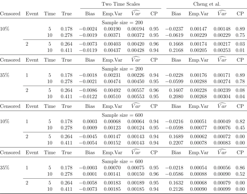
In the standard analysis of competing risks data, proportional hazards models for cause-specific hazards are fit using the same time scale for all causes of failure. We propose estimating cumulative incidence function by fitting regression models for the cause-specific hazard functions using different time scales for each cause. We establish consistency and asymptotic normality of the proposed estimator and assess its performance in simulations. The method is illustrated with stage III colon cancer data obtained from the Surveillance, Epidemiology, and End Results (SEER) program of National Cancer Institute.
TABLE OF CONTENTS
List of Tables . . . vi
List of Figures . . . vii
Chapter 1. Literature Review . . . 1
1.1 Introduction . . . 1
1.2 Overview of Competing Risks Data . . . 1
1.2.1 Non-Parametric Methods . . . 4
1.2.2 Semi-Parametric Methods . . . 4
1.3 Number Needed to Treat for Time To Event Data with Competing Risks . . 5
1.4 Endpoints for HIV Trials Measuring Viral Suppression and Multi-State Models 8 1.5 On the Choice of Time Scales in Competing Risks Predictions . . . 9
1.6 Competing Risks Data with Missing Cause of Failure . . . 11
Chapter 2. Number Needed to Treat for Time To Event Data with Competing Risks 14 2.1 Introduction . . . 14
2.2 Methods . . . 14
2.3 Tamoxifen Trial Example . . . 16
2.4 Practical Remarks . . . 21
Chapter 3. Combining Times to Suppression and Rebound in HIV Studies . . . . 23
3.1 Introduction . . . 23
3.2 Methods . . . 23
3.3 Simulation Results . . . 27
3.4 Re-analysis of the A5142 Trial . . . 32
3.5 Discussion . . . 35
Chapter 4. On the Choice of Time Scales in Competing Risks Predictions . . . 37
4.1 Introduction . . . 37
4.2 Methods . . . 37
4.3 Simulations . . . 41
4.4 Real Data Example . . . 47
4.5 Discussion . . . 52
4.6 Appendix . . . 53
Chapter 5. Non-Parametric Estimation of Cumulative Incidence Functions for Competing Risks data with Missing Cause of Failure . . . 59
5.1 Introduction . . . 59
5.3 Simulation Results . . . 67
5.4 Real Data Example . . . 73
5.5 Discussion . . . 75
5.6 Appendix 1 . . . 77
5.7 Appendix 2 . . . 92
LIST OF TABLES
3.1 Comparison of HIV endpoints in simulations . . . 31
3.2 Power computations results for proposed HIV endpoint . . . 32
3.3 Comparison of endpoints in re-analysis of A5142 trial . . . 34
4.4 Comparison of estimators on one and on two time scales - scenario 1 . . . 45
4.5 Comparison of estimators on one and on two time scales - scenario 2 . . . 46
4.6 Descriptive Statistics for SEER Data . . . 47
4.7 Regression coefficients from two models . . . 49
5.8 Performance of proposed method for missing cause of failure - scenario 1 . . 68
5.9 Performance of proposed method for missing cause of failure - scenario 2 . . 69
5.10 Comparison of variance estimators - scenario 1 . . . 70
LIST OF FIGURES
2.1 Probability of relapse and non-relapse death . . . 18
2.2 Non-parametric estimates of ARR and NNT . . . 19
2.3 Semi-parametric estimates of NNT . . . 20
2.4 Predicted NNT for specific covariate values . . . 22
3.5 Simulation scenarios for probability of suppression, rebound, and probability to be in suppression . . . 28
3.6 Survival function for composite endpoint and probability to be in suppression 33 4.7 Predicted cumulative incidences . . . 51
4.8 Baseline hazard compared to Gompertz distribution . . . 52
5.9 Probabilities of infection types, and of infection type being observed . . . 74
Chapter 1. Literature Review
1.1 Introduction
The intent of this dissertation proposal is to address various problems related to analysis of complex time-to-event data, such as competing risks data and multi-state models. The proposed dissertation will consist of 4 parts. The first part provides a simple extension of the definition of the number needed to treat to competing risks data. The second part defines a new alternative endpoint for clinical trials where the outcome is the time spent by a patient in some transient state, such as viral suppression in HIV clinical trials. The third part proposes an estimator for cumulative incidence functions under the competing risks setup, when a natural choice of time scales is different for different types of event. The final fourth part is dedicated to estimation of cumulative incidence functions under competing risks setup, when the information on the cause of failure is possibly missing.
1.2 Overview of Competing Risks Data
The difference between the classic time to event and competing risks settings is that instead of considering only one type of event, we now recognize that a patient can experience events of several types. One of them is the event of interest, but other events can happen too and they can affect our event of interest. An example of such data can be the tamoxifen trial described by Cummings et al (Cummings et al., 1993). In this trial data, we observe events of two types, a relapse and a death prior to relapse, with a relapse being the event of interest. Death before relapsing precludes a relapse from happening, and thus death prior to relapse is said to be a competing risk with respect to relapse.
Though the problem of dealing with competing risks data is a relatively old one, it is fair to say that there is no consensus about which function to choose to describe the probability of the event of interest. The two approaches most frequently used for this purpose are the cumulative incidence estimator and the complement of the Kaplan-Meier estimator (Kaplan and Meier, 1958). In our competing risks illustration above, the cu-mulative incidence function for relapse is Frelapse(t) = P r(T ≤ t ∧event type = relapse) and it is the probability of relapse in the existing conditions with competing risks present (Kalbfleisch and Prentice, 1980). The Kaplan-Meier estimator ˆSrelapse(t) estimates the func-tion Srelapse(t) = exp −Rt
0 λrelapse(u)du , where λrelapse(t) is the cause-specific hazard
function for relapse, formally defined below. Failures due to competing risks are treated by this estimator as censoring. In our example, a patient who died prior to experiencing a relapse would be considered censored.
Using the complement of the Kaplan-Meier estimator 1−Sˆ(t) still remains arguably the most common way to quantify the probability of the event of interest, even though there is much debate in literature about when it is appropriate. Some discussion on this topic and further references can be found in (Pepe and Mori, 1993) and (Gooley et al., 1999). It could be interpreted as the probability of the event of interest in a hypothetical situation when all the competing risks are removed, assuming that the events are independent (Tsiatis, 1975). That means that removing the mechanism which causes deaths prior to relapse would not affect the mechanism which causes relapse and hence the probability of relapse.
In general, 1−Sˆrelapse(t) is larger than the probability of the event of interest in the settings when all competing risks operate (Gooley et al., 1999). The reason why the results will be biased is that the Kaplan-Meier estimator treats patients who failed from competing causes the same way it treats censored, even though patients who were censored and those who failed from competing risks are very different on one particular respect. Patients who were censored can still experience the event of interest after being censored. In our example, if a patient was censored they still can experience a relapse in future, and we do take this possibility into account when we compute the probability of relapse. Patients who failed from a competing risk, however, cannot experience the event of interest any longer. A patient who died prior to relapse will never have a relapse. When we treat them the same way as we treat those who were censored and assume that they too have some non-zero probability to experience a relapse in future, we end up overestimating the probability of relapse when a competing risk of death prior to relapse is present. A formal yet very understandable mathematical explanation of this fact is given by Gooley in (Gooley et al., 1999).
denote the type of event, ∈ {1, ..., J}, T the time of event, and C – the censoring time. Also, let Z be a p×1 vector covariates, possibly time-dependent. The distribution of time to the event of interest may depend on the covariates, so we may be interested in being able to adjust for covariate values during estimation.
Suppose we have N patients, indexed by i = 1, . . . , N. The data we observe for the
i-th patient is (Xi, δi, i,Zi), where Xi = min(Ti, Ci), δi = I(Xi = Ti), and i – the event type. The random variable i is not observed if δi = 0. We assume that (Xi, δi, i,Zi),, are independent and identically distributed, and that the censoring mechanism is independent of the mechanisms that cause events, conditionally on covariates values in Z.
We define the cumulative incidence function, or subdistribution, for an event of type j,
j = 1, ..., J, as Fj(t;Z) = P r(T ≤ t, = j | Z), which is the probability an event of type j occurs by the time t.
There are two types of hazard functions which we can use to describe the competing risks data. One is the cause-specific hazards, defined as:
˜
λj(t;Z) = lim
∆t→0
1
∆tP r{t≤T ≤t+ ∆t, =j |T ≥t,Z}
(1.1) This function can be viewed as an instantaneous rate of event type j given a patient being at risk, with ‘being at risk’ defined as not having experienced any event by the time t.
A subdistributional hazard function λj(t;Z) for the event of type j is
λj(t;Z) = lim
∆t→0
1
∆tP r{t≤T ≤t+ ∆t, =j |T ≥t∨(T ≤t∧6=j),Z}
= d
dtFj(t;Z) 1−Fj(t;Z)
Note that for the purpose of this second definition ‘being at risk’ defined as not having experienced an event of type j. Thus a patient who has experienced a competing event of type 2 still is considered to be at risk for an event of type 1.
The cumulative incidence function can be expressed via cause-specific hazard functions as:
Fj(t;z0) = t Z
0
S(u)˜λj(t;Z))du}.
subdistri-butional hazard function as
Fj(t;z0) = 1−exp{− t Z
0
λj(u;z0)du}.
1.2.1 Non-Parametric Methods
Let t1 ≤t2 ≤ . . .≤ tn be the ordered observed times when an event of any type occurred. Let dij be the number of events of type j that occurred at time ti. Let yi be the number of patients who are still at risk just prior to time ti, that is those who haven’t experienced any event and haven’t been censored yet. Let S(t) =P r(T ≥t) denote the overall survival function, which is the probability of surviving to the time t without experiencing an event of any type. The non-parametric estimate of the cumulative incidence function is given by the Aalen-Johansen estimator (Aalen and Johansen, 1978):
ˆ
F1(t) =
X
ti≤t
ˆ
S(ti−)
di1
yi
where ˆS(·) is the Kaplan-Meier estimator of the overall survival function.
There exist a number of estimators for the variance of ˆF1(t). A comparison of their
empirical performance in small samples is given in (Braun and Yuan, 2007). The following variance estimator is obtained by simplifying the Gray’s estimator (Gray, 1988) for the case of competing events of two types:
d
V ar( ˆF1(t)) =
X
ti≤t
{Fˆ1(t)−Fˆ1(ti)−Sˆ(ti)}2
di1
y2
i
+X
ti≤t
{Fˆ1(t)−Fˆ1(ti)}2
di2
y2
i
.
1.2.2 Semi-Parametric Methods
When it is desirable to look at the effect of covariates on the treatment effect, a semi-parametric approach can be used. One can model either the cause-specific hazard functions, or subdistributional hazards.
Fine and Gray in (Fine and Gray, 1999) developed the proportional subdistributional hazards model which states that
λ1(t;Z) =λ10(t) exp{ZT(t)β0}
where λ10(t) is the baseline subdistributional hazard function and β0 is a p×1 parameter
vector. If the covariate vector Z(t) = Z does not depend on time, the subdistributional hazards are proportional for all values oft. In the general case, we allow for time×covariate interactions, and hence for time-dependent covariates. The cumulative incidenceF1(t;Z) can
then be expressed as
F1(t;Z) = 1−exp
−
t Z
0
λ10(s) exp{ZT(s)β0}ds
,
from which one can estimate the parameter vector ˆβ using the modified score function from the partial likelihood for F1(t;Z) (Fine and Gray, 1999), and the baseline integrated hazard
for subdistribution ˆΛ10(t) by a modification of Breslow’s estimator (Breslow, 1972).
For a given value of a covariate vector Z=z0 we can compute the integrated hazard
ˆ
Λ1(t;z0) = t Z
0
exp{z0(s) ˆβ}dΛˆ10(s)
and the predicted cumulative incidence function as ˆ
F1(t;z0) = 1−exp{−Λˆ1(t;z0)}.
1.3 Number Needed to Treat for Time To Event Data with Competing Risks
expected event under Treatment than Control, defined formally by N N T(πCtl −πT rt) = 1 or, equivalently,
N N T = 1
πCtl−πT rt.
The denominator is known to epidemiologists as the risk difference (RD), absolute risk (AR), or absolute risk reduction (ARR) (Last, 1988; Cook and Sackett, 1995); succinctly, we write
N N T =ARR−1. The more efficient a treatment, the greater the ARR and the smaller the NNT. This simplicity of interpretation facilitates use of NNT in communicating the practical impact of a treatment effect on a scale more readily accessible to health care providers and patients than either absolute or relative risk. The clinical trial-based definition of NNT may be extended to communicate the potential benefits of a preventive behavior or public policy change, by replacing control and treatment groups in the clinical trial setting with higher and lower levels of a modifiable exposure in a field trial or observational study. Although caution is clearly required when interpreting NNT from non-experimental data, in such contexts
ARR−1 may be interpreted as the “number needed to prevent” if the exposure is assumed to be causal.
To estimate the NNT, one needs respective estimates ˆπT rt,πˆCtl of πT rt, πCtl, from which a point estimate ARR[ = (ˆπCtl −πˆT rt) of ARR immediately follows, and a 100(1−α)% confidence interval (ARRL, ARRU) may be obtained using a number of methods (Connor and Imrey, 2005). From these we obtain corresponding point estimate N N T\ =ARR[−1 and 100(1−α)% confidence interval (N N TL, N N TU) = (ARR−U1, ARR
−1
L ) for the NNT.
Some technical challenges in reporting and interpreting the NNT and its confidence in-terval arise when the difference in the event rates between the groups is not statistically significant. In this case the confidence interval for the absolute risk reduction contains zero and its lower limit is negative. Therefore, the confidence interval for the NNT will contain infinity and have a form (−∞;−a]∪[b;∞) for some a > 0, b > 0. The interpretation of the negative part of this confidence interval may be the number of patients who need to be treated in order to observe one event more in the treatment group compared to the control group, which is sometimes referred to as “the number needed to harm” (or NNH), which nat-urally arises when evaluating side effects of therapies (Altman, 1998). McQuay and Moore in (McQuay and Moore, 1997) suggest that in such cases only the point estimate without the confidence interval be reported. However, we will report such confidence intervals, because they can convey information useful for decision-making in clinical settings.
person-time denominated constant N N T∗ = (λCtl −λT rt)−1 can be used as an underlying and simpler summary of treatment impact than the full NNT function. Under these circum-stances, the survival functions are declining exponentials, with their complements πCtl, πT rt thus respectively well-approximated for sufficiently low t bytλCtl, tλT rt; this yields the sim-ple approximation N N T(t) ∼ N N T∗/t. The hazards may be estimated in each group as the ratio of total events to total person-time monitored. Confidence intervals for N N T∗
may be formed based on the Poisson distribution if patients and time are both assumed homogeneous, and on the negative binomial or other model to take patient heterogeneity into account.
However, when hazard rates vary during the intervals in which patients are observed, the ARR computed from the average incidence densities and the NNT taken as its inverse do not accurately describe the trajectory of treatment or exposure impact over time, and may be seriously misleading. For such time-to-event studies, which thus require survival analysis, Altman and Andersen (Altman and Andersen, 1999) have defined the NNT in the clinical trial context as a function of time:
N N T(t) = 1
ST rt(t)−SCtl(t)
where ST rt(t), SCtl(t) are the probabilities to survive without an event up to time t in the treatment and control groups respectively. Often only a few given points in time would be of practical interest. Altman and Andersen (Altman and Andersen, 1999) suggested methods to obtain estimates and confidence intervals for the NNT(t) from published results of clinical trials with time to event data when either non-parametric or semi-parametric analysis had been performed. Obviously, if raw data are available, NNT(t) can be estimated easily using the same methods.
as death from myocardial infarction, complications of diabetes, other types of cancer etc., which makes tools developed for a competing risks setup most appropriate for analysis of the trial data. However, if one wished to quantify the benefits of tamoxifen demonstrated by this trial using NNT(t), one would face the problem that the NNT(t) defined for standard time to event settings may not be appropriate and that no definition of NNT(t) for data with competing risks exists. Chapter 2 of this dissertation suggests such a definition.
1.4 Endpoints for HIV Trials Measuring Viral Suppression and Multi-State
Models
A well-defined outcome is fundamental to the analysis of time to event data. However, in some settings a clear definition of the event of interest is a challenge. An example of such settings are prospective studies, including recent clinical trials evaluating the difference between treatments or exposures which are intended to suppress the level of HIV-1 RNA viral load (henceforth viral load) in people infected with HIV.
Infection with HIV is monitored by the number of copies of viral load present in circulating plasma (Mellors et al., 1996). The level and change in viral load is an important indicator of HIV disease progression. HIV research relies heavily on viral load levels for evaluating the comparative efficacy and effectiveness of competing therapy regimens, and estimating the prognosis of HIV-infected individuals (Egger et al., 2002; Cole et al., 2007; Riddler et al., 2008). The relative performance of HIV treatments depends on the combination of how quickly and to what extent the treatment suppresses viral load, and how well a treatment maintains a suppressed viral load.
arbitrarily (by the choice of m) redefine the time of event, which can have a notable impact on results, as evidenced in the simulation studies further in this document, in Chapter 3, Section 3.3.
To avoid the above mentioned problems, we suggest the use of a different endpoint and different analysis methods based on non-parametric methods for multi-state models developed by Pepe (Pepe, 1991). The methods have been developed for the situation when each patient can experience not one but several distinct events of types j, j = 1, ..., J. The event of each type can be experienced only once. The data from each patient has a form of (Tji), whereTji is the time of eventjfor thei−thpatient. For each of the event types we can define estimators of individual cumulative incidence functions ˆFj(t). For a smooth function
g of several such estimators, Pepe derives the asymptotic properties of the resulting quantity and proposes a two-sample weighted test statistic for it. Using our illustration from the Section 1.2, if the event of type 1 is the suppression of the viral load, and the event of type 2 is the rebound of the viral load, withF1(t), F2(t) being their cumulative incidence functions,
then we can define the probability that a patient’s viral load is suppressed at a given time t
asP rsuppr(t) =F1(t)−F2(t) =g(F1(t), F2(t)), with function g being g(a, b) =a−b. We can
obtain the standard error SEc(P rcsuppr(t)), and, further, we can construct a test statistic, if we have two groups of patients and wish to compare the probability of a patient’s viral load being suppressed between these two groups.
1.5 On the Choice of Time Scales in Competing Risks Predictions
in Cheng et al (Cheng et al., 1998) :
ˆ
Fj(t|z0)) =
t Z
0
ˆ
S(u|z0)dΛˆj(u|z0)
where
ˆ
S(u|z0) = exp{−
J X
j=1
ˆ
Λj(u|z0)},
ˆ
Λj(u|z0) = ˆΛ0j(u)exp( ˆβjz0),
ˆ
Λ0j(u) = n X
i=1
δjiI(Xi ≤u)
n X
k=1
I(Xi ≤Xk)exp(βjZk)
−1
,
1.6 Competing Risks Data with Missing Cause of Failure
As it was described above in Section 1.2, an essential component of competing risks data is the cause of each observed failure, denoted by i. However, in practice the cause of failure is often unknown, either at all or at the moment of data analysis. For example, in an on-going cohort study with follow-up, the fact and date of death may be known from follow-up calls or from obituaries, but the properly adjudicated cause of death for some patients may become available with a significant lag time and thus be missing at the time of data analysis. Alternatively, if an autopsy was not performed, it may be not possible to classify a death as a cancer-related or a non-cancer death. There have been suggested numerous methods to analyse competing risks data with possible missing cause of failure.
In 1982 Dinse (Dinse, 1982) provided a classification of incomplete competing risks data, which along with the standard fully observed and fully censored observations allowed two kinds of partially complete observations, with either observed time of failure and missing type of failure, or with an observed type but censored time of failure. To analyse such data, he suggested a non-parametric maximum likelihood estimator (NPMLE) obtained by an EM algorithm, which reduced to a closed-form estimator in case the data contained no observations with observed failure type and censored failure time. The estimated quantities were the overall survival function and the time-dependent probabilities πj(tk) of having an failure of a type j, given the fact of the failure in the time interval [tk, tk+1) (the time in
his analysis was discrete and thus there were more than one event in each interval). The proposed estimator for πj(tk) was a proportion of failures of type j among all failures with known type that had occurred during the time interval and did not involve any smoothing which made the estimates ”extremely erratic”, though, interestingly, smoothing was used for display purposes in figures. The missingnes of the cause of failure was assumed to be independent of the type of failure. In a subsequent paper (Dinse, 1986), Dinse suggested another EM algorithm, for the case when time of event is always observed but the probability of the type of failure being observed depends on the type of failure.
Racine-Poon and Hoel (Racine-Poon and Hoel, 1984) considered non-parametric estima-tion of net survival funcestima-tions Sj(t) = exp(−
t R
0
λj(u)du) for data with exactly two mutually exclusive causes of failure where the cause of failure was determined only with some degree of certainty. Unlike in the standard competing risks setup, their data consisted of pairs (Ti, Pi) where Ti is the time of failure as usual, and Pi is the probability that the failure of subject
estimator of the overall hazard function, and ˆπ1(Ti) was taken to be equal toPi.
Miyakawa (Miyakawa, 1984) studied a fully parametric exponential model and a non-parametric model, both under the MCAR assumption for the missing type of failure. For the non-parametric case, he suggested yet another version of an EM algorithm. At each estimation step, the probabilities of failure of type 1 were expressed as ˆλ1(t)/[ˆλ1(t) + ˆλ2(t)]
where ˆλj(t), j = 1,2,were obtained as a simplest local constant smoothers from the Kaplan-Meyer-type estimates of the net survival functions.
Lo (Lo, 1991) regarded a competing cause of failure as censoring, with the censoring indicator possibly missing, and suggested two NPMLE estimators for the case when the probability of the censoring indicator to be observed was the same for all subjects and con-stant over time. The first one used all observations, and the contribution to the likelihood from the observations with the missing censoring indicator was weighted by the proportion of uncensored events π(t). The estimates ˆπ(t) could be viewed as being smoothed over the tail of the distribution of t. The second estimator introduced a simplest inverse probabil-ity weighting scheme, where only the fully observed data was used in the Kaplan-Meyer estimator, but contributions of all complete case observations were weighted by the inverse probability of the censoring indicator being observed (which was assumed constant).
The topic has been extensively explored since. Goetghebeur and Ryan (Goetghebeur and Ryan, 1990) proposed a modification of the logrank test for competing risks with missing cause of failure, which was further developed by Dewanji (Dewanji, 1992). Semi-parametric estimators were developed by Gijbels, Lin, and Ying (Gijbels et al., 1993), Goetghebeur and Ryan in the 1995 paper (Goetghebeur and Ryan, 1995), Gao and Tsiatis (Gao and Tsiatis, 2005). Lu and Tsiatis (Lu and Tsiatis, 2001) suggested using multiple imputations for the missing event type, based on a parametric model for the conditional probability of the event of interest given that an event of any type has occurred. The problem of time-to-event data without competing risks but with possibly missing censoring indicator was further studied by McKeague and Subramanian (McKeague and Subramanian, 1998). Yet another version of the problem was addressed by Craiu and Duchesne (Craiu and Duchesne, 2004) and Craiu and Reiser (Craiu and Reiser, 2006). They considered competing risks data with masked event types, that is for some subjects the event type could be determined only up to some subset of all possible event types.
Chapter 2. Number Needed to Treat for Time To Event Data with Competing
Risks
2.1 Introduction
The intent of this chapter is to propose methods to define the number needed to treat for time to event data in presence of competing risks and to estimate it from the raw data using both non-parametric and semi-parametric approaches. This is done in Section 2.2. The methods are illustrated on the breast cancer data in Section 2.3 with some practical remarks concluding in Section 2.4. The work has been published (Gouskova et al., 2014b).
2.2 Methods
We will use the notation introduced in the Chapter 1 above. For purposes of this chapter it is sufficient to consider events of only two types, 1 and 2, with type 1 the event of primary interest and type 2 the competing risk. If more than one competing risk is present, then we can combine them all into one type of event without loss of generality. The non-parametric and semi-non-parametric methods discussed below are not sensitive to the grouping of the competing events.
Let us denote the cumulative incidence function for an event of type j for j = 1,2 as
Fj(t;Z) = P r(T ≤ t, = j |Z). In the sequel, we will let superscripts T rt and Ctl denote the membership in the treatment and control groups respectively.
We define the NNT with respect to the event of type 1 as follows:
N N T1(t;Z) =
1
ARR1(t;Z)
where
ARR1(t;Z) = F1Ctl(t;Z)−F
T rt
1 (t;Z)
is the absolute risk reduction from the subdistribution.
To obtain a point estimate of N N T1(t;Z) we need estimates ofF1Ctl(t;Z) and F1T rt(t;Z),
which can be obtained by using various methods. We will discuss the details of using non-parametric and semi-non-parametric methods in the corresponding sections below.
informa-tion useful for decision-making in clinical settings. Estimating the confidence interval for the NNT is therefore a two-stage process. First, we estimate the ARR1(t;Z), obtain its
confidence interval and determine if the ARR is significantly greater than zero. Second, if the ARR is significantly greater than zero, then the confidence interval for the NNT is [1/ARRU(t); 1/ARRL(t)], where 0 < 1/ARRU(t) < 1/ARRL(t). If the ARR is not signifi-cantly greater than zero, then we report two confidence intervals, [1/ARRU(t),∞) for the NNT and [−1/ARRL(t),∞) for the NNH, whereARRU(t)>0 andARRL(t)<0.
Under the non-parametric approach, the cumulative incidence function is estimated sep-arately for the treatment and the control groups. Since we assume that all patients are independent, the estimates of the cumulative incidence functions in the treatment and the control groups are independent and the covariance between them is equal to zero. Hence the variance of the ARR\1(t) is
V ar(ARR\1(t)) =V ar( ˆF1Ctl(t)) +V ar( ˆF
T rt
1 (t))
The 95% confidence interval for ARR\1(t) is given by [ARRL(t);ARRU(t)] where
ARRL(t) =ARR\1(t)−1.96·
q
(V ard(ARR\1(t)) and ARRU(t) = ARR\1(t)+1.96· q
d
V ar(ARR\1(t).
The point estimate and the confidence interval for the NNT can be computed now as de-scribed above.
When it is desirable to look at the effect of covariates on the treatment effect, a semi-parametric approach can be used. Any method allowing estimation of the cumulative in-cidence function given covariate values can be used for the purpose of the definition of the NNT.
For example, we can use the Fine and Gray model (Fine and Gray, 1999). When one of the covariates, say z0p, is the treatment group assignment, 1 for the active treatment and 0 - for control, we can compute the cumulative incidence functions for the treatment and control groups as
ˆ
F1T rt(t;z00) = ˆF1(t;z00, z0p = 1) ˆ
F1Ctl(t;z00) = ˆF1(t;z00, z0p = 0)
where z00 = (z01, ..., z0,p−1)T is the vector of covariates other than treatment group. Having
those, we can compute the point estimate for the ARR(t;z00) and NNT(t;z00).
semi-parametric than for the non-semi-parametric approach, because in this case we use all of the observations to estimate of both F1T rt(t;z00) and F1Ctl(t;z00). Hence, the estimates of the cumulative incidence functions ˆFT rt
1 (t;z
0
0) and ˆF1Ctl(t;z 0
0) in the treatment and the control groups are no longer independent. Therefore to compute the variance of the ARR(t;z00) we need the covariance between ˆFT rt
1 (t;z
0
0) and ˆF1Ctl(t;z 0
0), for which no simple closed form is known. This challenge is the same as for computing the confidence intervals for the number needed to treat for classic time to event data without competing risks, described by Altman and Andersen in (Altman and Andersen, 1999).
A practical solution is to obtain the variance of the ARR(t;z00) via bootstrapping. To do this, at each repetition of the bootstrapping process, we draw two bootstrap samples independently, one from the treatment group and the other from the control group, combine them into a single bootstrap sample, re-fit the model to the combined bootstrap sample and compute the ARR estimate, and after repeating the procedure the desired number of times compute the estimator of the variance of the ARR[(t;z00) from all of the bootstrap samples. A more general direct regression model for the cumulative incidence function was sug-gested by Fine (Fine, 2001). This includes alternatives to the proportional subdistribution hazards model. Klein et al. (Klein et al., 2007) proposed fitting such models using a pseudo-value approach. In particular, if we are interested in fitting such a model at a specific time point t0 of interest, such as 5 years after the treatment, we let ˆF1(t0) =Pti≤t0
ˆ
S(ti−)dyi1
i be
the non-parametric estimate of the cumulative incidence function from the whole sample as defined in Section 3.1 above, and ˆF1(j)(t0) be the same estimate computed with the j −th
observation removed from the sample. Defining the pseudo-observations for the cumulative incidence function as ˆθj =nFˆ1(t0)−(n−1) ˆF
(j)
1 (t0),one may estimate the generalized linear
model E(ˆθj|Zj) proposed by Fine (Fine, 2001) using a generalized estimating equations ap-proach. As an example, assuming a linear model for the cumulative incidence function with an identity link and employing a working independence covariance matrix, the estimate of the ARR reduces to ARR[(t0;z00) =−βˆp. The variance of ˆβp and hence confidence intervals for the ARR can be obtained as described in (Klein et al., 2007). The point estimate and the confidence interval for the NNT as a function of time can now be computed as described just prior to Section 3.1.
2.3 Tamoxifen Trial Example
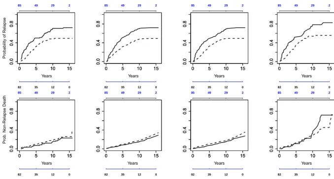
the 10-week period before entry into the trial. The data used in this example consist of the observations on 167 eligible patients of the trial, 82 of whom were randomized to placebo and 85 to tamoxifen treatment. The median observation period for these patients was 5.06 years (range from 0.14 to 15.95 years). Of the patients in the placebo group, 59 experienced a recurrence of breast cancer and 19 died without relapse from other causes. In the active treatment group, 42 had a relapse and 23 died without recurrence. The data available for each patient also includes age at time of randomization (ranging from 65 to 84, with median age 71), tumor size (from 3 to 170 mm, median 25), and the number of positive nodes (from 1 to 34, median 3). The last relapse occurred in the control group at 13.16 years, and the last non-relapse death - in the tamoxifen group at 15.7 years, as can be seen in the non-parametric plots in Figure 2.1.
We computed the NNT based on these data using non-parametric and semi-parametric approaches. The choice of a semi-parametric model and model diagnostics were discussed in detail in (Fine and Gray, 1999). Here we will only mention briefly that the proportional hazards model λ1(t;Z) =λ10(t) exp(β0Z) does not fit the data well, and a semi-parametric
model allowing the hazard ratio to be quadratic in time, λ1(t;Z) =λ10(t) exp(β0Z+β1Zt+
β2Zt2), is a more appropriate choice.
Figure 2.1 shows different estimates of the probability of relapse and non-relapse death by treatment group: the estimates of cumulative incidence functions obtained by using the three models, non-parametric, semi-parametric with proportional subdistributional hazards, and semi-parametric with the quadratic in time hazard ratio, along with the complements of the Kaplan-Meier estimator for comparison. As one can see, the estimates of the cumulative incidence functions for the non-relapse death are very close in both groups and don’t differ much across the three analysis methods. The estimates are slightly higher in the tamoxifen group. The estimated cumulative incidence functions for relapse differ noticeably between the two treatment groups, with higher estimates in the control group.
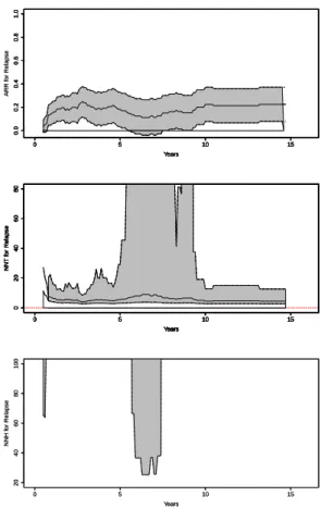
Figure 2.2 shows the plot of the non-parametric estimates of the absolute risk reduction and the NNT, both accompanied by pointwise 95% confidence regions. The ARR was not significantly different than zero around 6 months and between 5.5 and 7.5 years (as seen on the plot, the lower confidence limit is negative), therefore the pointwise confidence regions for the NNT around 6 months and between 5.5 and 7.5 years consist of two parts and include infinity. We plotted the negative part of confidence regions for the NNT in a separate panel, as the number needed to harm (NNH).
0 5 10 15
0.0
0.4
0.8
Years
Probability of Relapse
0 5 10 15
0.0
0.4
0.8
82 35 12 0
85 49 29 2
0 5 10 15
0.0
0.4
0.8
Years
0 5 10 15
0.0
0.4
0.8
82 35 12 0
85 49 29 2
0 5 10 15
0.0
0.4
0.8
Years
0 5 10 15
0.0
0.4
0.8
82 35 12 0
85 49 29 2
0 5 10 15
0.0
0.4
0.8
Years
0 5 10 15
0.0
0.4
0.8
82 35 12 0
85 49 29 2
0 5 10 15
0.0 0.4 0.8 Years Prob . N on-Relapse D eath
0 5 10 15
0.0
0.4
0.8
82 35 12 0
85 49 29 2
0 5 10 15
0.0
0.4
0.8
Years
0 5 10 15
0.0
0.4
0.8
82 35 12 0
85 49 29 2
0 5 10 15
0.0
0.4
0.8
Years
0 5 10 15
0.0
0.4
0.8
82 35 12 0
85 49 29 2
0 5 10 15
0.0
0.4
0.8
Years
0 5 10 15
0.0
0.4
0.8
82 35 12 0
85 49 29 2
Figure 2.1: Probability of relapse (top row) and non-relapse death (bottom row). Col-umn 1: cumulative incidence, non-parametric model; ColCol-umn 2: cumulative incidence, semi-parametric proportional hazards; Column 3: cumulative incidence, semi-parametric quadratic in time; Column 4: complement of the Kaplan-Meier estimator. (Solid line - con-trol group, dashed line - tamoxifen group. Number at risk for tamoxifen group - above each
0 5 10 15 0.0 0.2 0.4 0.6 0.8 1.0 Years ARR f or Relapse
0 5 10 15
0.0 0.2 0.4 0.6 0.8 1.0 Years ARR f or Relapse
0 5 10 15
0.0 0.2 0.4 0.6 0.8 1.0 Years
0 5 10 15
0.0 0.2 0.4 0.6 0.8 1.0 Years
0 5 10 15
0 20 40 60 80 Years NNT f or Relapse
0 5 10 15
0 20 40 60 80 Years NNT f or Relapse
0 5 10 15
0 20 40 60 80 Years NNT f or Relapse
0 5 10 15
0 20 40 60 80 Years NNT f or Relapse
0 5 10 15
0 20 40 60 80 Years NNT f or Relapse
0 5 10 15
0 20 40 60 80 Years NNT f or Relapse
0 5 10 15
20 40 60 80 100 Years NNH f or Relapse
0 5 10 15
20 40 60 80 100 Years NNH f or Relapse
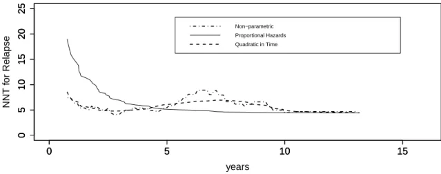
in Section 3.2, and the time-quadratic generalization considered in (Fine and Gray, 1999) and noted above. The non-parametric NNT function and its counterpart from the semi-parametric model with quadratic in time hazard ratio behave very similarly, especially at the early times between 0.5 and 4 years and in the tail after 8 years. The NNT function from the semi-parametric proportional hazards subdistributional model without covariate× time interaction terms differs from these two models very noticeably early, overestimating the NNT prior to 4 years, and does not reflect the non-parametric function’s local maximum around 6-7 years. Beyond 10 years, however, all three estimates are very similar. For example, at 12 years the non-parametric estimate is 4.69 with 95% confidence interval [2.78; 15.09], the estimate from proportional hazards model is 4.41 with 95% confidence interval [2.73; 11.45], and the estimate from quadratic in time model is 4.70 with 95% confidence interval [2.76; 15.72]. The more optimistic point estimate and upper confidence interval limit from the proportional hazards model appear to reflect oversmoothing by the proportional hazards model in the 5-10 year period, visible in Figure 2.1.
0 5 10 15
0
5
10
15
20
25
years
0 5 10 15
0
5
10
15
20
25
0 5 10 15
0
5
10
15
20
25
NNT f
or Relapse
Non−parametric Proportional Hazards Quadratic in Time
Figure 2.3: Estimates of the NNT for non-parametric, semi-parametric proportional hazards, and semi-parametric quadratic in time models.
Hence, a single time point at 12 years after the beginning of the treatment might be an appropriate choice, after which the rate of relapse is rather low. At 12 years after mastectomy, the patients who received tamoxifen as a post-operative treatment experienced substantially fewer breast cancer recurrences compared to those who were on placebo. The reduction in the probability of relapse corresponds to one event of relapse in approximately every 5 patients treated, with a 95% confidence interval approximately 3 to 16.
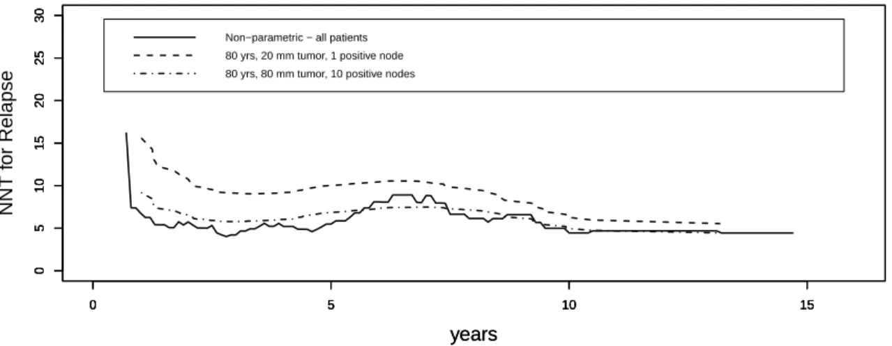
It may also be useful to estimate the NNT for a specific subgroup of patients, e.g., based on age and disease severity. To do this, we included age, tumor size, and the logarithm of number of positive nodes, in addition to the treatment group, as time-independent covariates. Age had no significant effect on the distribution of time to relapse. Figure 2.4 compares the predicted NNT computed for an 80-year-old patient with the tumor size 20 mm and 1 positive node with the NNT for an 80-year-old patient with the tumor size 80 mm and 10 positive nodes. The non-parametric NNT computed from the data of all the patients is also given as a reference. The estimated NNT is lower for a patient at a more severe stage of disease, indicating greater treatment effect. This makes sense because one expects the relapse probability for any given time from mastectomy to be lower, in both tamoxifen and control groups, among patients initially treated at earlier vs. later stages of breast cancer. This lower baseline risk at earlier disease stages limits the potential absolute tamoxifen benefit, and the absolute impact of a constant relative benefit will be less pronounced than among patients with diagnosis and surgery later in the disease course. The difference between subgroups is greater in the short run and attenuates by 12 years.
We also performed an analysis similar to that described above, but with death prior to relapse as the event of interest. Other than age, no covariates, including treatment group, had any statistically significant effect on the distribution of the time to non-relapse death. There was no significant difference in the probability of the non-relapse death between the tamoxifen and placebo groups at any time point, regardless of which method was used to compute the estimates. To ascertain the sensitivity of the analysis of these data to treating death without relapse as a competing risk rather than as an independent censoring mechanism, we computed the NNT(t) using the complement of the Kaplan-Meier estimators instead of the cumulative incidence functions as estimates of the probabilities of relapse. For these data, results changed little.
2.4 Practical Remarks
0 5 10 15
0
5
10
15
20
25
30
years
NNT f
or Relapse
0 5 10 15
0
5
10
15
20
25
30
0 5 10 15
0
5
10
15
20
25
30
years
Non−parametric − all patients 80 yrs, 20 mm tumor, 1 positive node 80 yrs, 80 mm tumor, 10 positive nodes
Figure 2.4: Estimates of the NNT for subgroups with specific values of covariates.
Chapter 3. Combining Times to Suppression and Rebound in HIV Studies
3.1 Introduction
The goal of this chapter is the development of an endpoint which is tailored to the objectives of HIV-1 and similar studies and provides an intuitive summary of treatment differences.
As mentioned earlier in Chapter 1, Section 1.4, the endpoints currently used to assess the suppression of the viral load in HIV studies may suffer from some problems. To avoid these problems, we suggest using a different endpoint and different analysis methods based on multi-state models (Pepe, 1991). These methods explicitly acknowledge the fact that we have two distinct events, viral load suppression and rebound, with corresponding survival functionsSS(t) andSR(t) respectively. Our proposed endpoint is based on the probability of being in suppression G(t), which is simply SR(t)−SS(t). We suggest an intuitive summary of treatment efficacy based on a weighted integral of this difference over a specified time interval of interest, say one year. With equal weights over time, this measure reduces to the restricted mean time suppressed over the time interval. One may tailor the weights to emphasize the timepoints of scientific interest, enabling a rigorous exploration of either early or late suppression dynamics. This endpoint is well-defined and has a clear and simple interpretation which may permit comparisons across trials and populations. The proposed analysis accounts for the fact that a proportion of patients will never suppress their viral load and allows investigators to simultaneously assess differences in both time to viral suppression and time to viral rebound, emphasizing those timepoints relevant to treatment evaluation.
The proposed endpoint is described in Section 3.2. A simulation study assessing perfor-mance of the proposed endpoint in comparison to endpoints based on composite events is discussed in Section 3.3. The practical utility of the analysis is illustrated in a reanalysis of ACTG A5142 in Section 3.4. A discussion concludes in Section 3.5. The work has been accepted for publication (Gouskova et al., 2014a).
3.2 Methods
For patient i, let Ri be the treatment regimen assignment at time of randomization, with the focus being an intent to treat analysis of treatment efficacy. The potential time at which patient i has their viral load suppressed is denoted by TS
i and the potential time at which patient i has their viral load rebound is denoted by TiR. Let Ci denote the potential censoring time for patienti, with the binary indicatorsδSi andδiRequal to 1 whenTiS andTiR
and XiR=min(TiR, Ci). In general,δiS ≥δRi , because the time to rebound of viral load may only occur subsequent to viral load suppression. For patient i, the observed data consists of (XS
i , δiS, XiR, δiR, Ri). The main difficulty in conducting a time-to-event intent to treat analysis using this data structure is that there is not an obvious single ”time to event” on which to base the analysis.
Suppose for simplicity that there are two treatment groups, r = 1 and 2, and let SS r and SrR denote the survival functions for TiS and TiR, respectively, in group r = 1,2. The endpoint we propose for viral suppression studies is the probability of being suppressed at time t, Gr(t) = SrR(t)− SrS(t), r = 1,2. This endpoint is defined without conditioning on information observed post randomization and may be analyzed using intent to treat methods. However, because the event probability is the difference of two survival functions and is not itself a survival function for a single time to event, the Kaplan-Meier estimator and logrank test are not applicable. Inferential methods for multi-state data must be used in the development of non-parametric estimators and tests for treatment differences.
Following (Pepe, 1991), we employ the Kaplan-Meier estimates ˆSrS(t),SˆrR(t),r = 1,2, of survival functions for time to viral suppression and time to viral rebound respectively. Note that time to viral rebound defined as above is measured from randomization. The survival function for time to viral rebound will be the marginal survival function, not conditional on being suppressed. We can estimate the probability for a patient to be in the state of suppression, within each treatment group separately, as
ˆ
Gr(t) = ˆSrR(t)−Sˆ S
r(t) for r= 1,2. The variance estimator for ˆGr(t), r= 1,2, is given by
d
V ar( ˆGr(t)) = 1
n2
r X
i:Ri=r
[ ˆXGir(t)]2
where nr is the number of subjects in group r,
ˆ
XGi
r(t) =nr
ˆ
SrS(t){ t Z
0
1
YS(u)
dNSi − t Z
0
Yi S(u) (YS(u))2
dNS(u)}−
−nrSˆrR(t){ t Z
0
1
YR(u)
dNRi − t Z
0
Yi R(u) (YR(u))2
dNR(u)},
re-spectively for a patient i, YSi(u) and YRi(u) are the at risk processes for suppression and rebound respectively for a patient i, and
Y(u) = X i:Ri=r
Yi(u) and N(u) = X i:Ri=r
Ni(u) for ∈ {S, R}.
The probability of being in suppressionGr(t) for groupr= 1,2 varies over time, similarly to a survival function, albeit not a monotonically decreasing function oft. As with standard time to event analyses, simple summary measures are needed for quantifying differences among treatment regimens. One should recognize that Gr(t) does not have a corresponding hazard function and treatment differences cannot be summarized using hazard ratios, as they might in separate analyses of SR
r and SrS. We suggest summarizing using the weighted restricted mean time a patient from group r will spend in suppression in the time interval [0, t0], which is
Rt0
0 Wˆ(u)Gr(u)du, where ˆW(u) is an estimate of some appropriately chosen
weight functionW(u) discussed below.
The analysis may be tailored to capture the information of greatest importance with a careful choice of the weight function. When W(u) ≡1, the weighted integral estimates the restricted mean time spent in viral suppression. For those interested in short term outcomes, larger weights may be applied at early time points, and vice versa for long term outcomes. For example, for those interested primarily in long term maintenance, zero weights may be employed at time points before some predetermined cut-off for suppression, eg 24 weeks. On the other hand, for those interested in population health where individuals with circulating virus present a transmission risk, non-zero weights at early time points would be an important consideration.
Following (Pepe, 1991), for the purpose of hypothesis testing one may compute a simple Z type test statistic as the difference of the weighted averages in the two treatment arms. The test statistic is:
W G=
r
n1n2
n1 +n2
t0
Z
0
ˆ
W(u){Gˆ1(u)−Gˆ2(u)}du.
Under the null hypothesis, the test statistic is asymptotically normal with zero mean and its asymptotic variance can be estimated by
d
V ar(W G) = n1n2
n1+n2
where
b
Vr = 1
n2
r X
j:Rj=r
t0
Z
0
ˆ
W(u) ˆXGj rdu
2
, r= 1,2.
Wald type confidence intervals for the weighted average time in suppression may be calculated using the asymptotic normality of the estimatorRt0
0 Wˆ(u) ˆGr(u)duand its variance estimator
ˆ
Vr, r= 1,2.
The choice of the weight function may also be directed towards improving the power of the test statistic to detect treatment differences in the probability of suppression over time. As suggested by Pepe and Fleming (1989), one may downweight at time points where
ˆ
G1−Gˆ2 is highly variable using the weight function:
ˆ
Wse(u) = 1/SEˆ [ ˆG1(u)−Gˆ2(u)],
where SEc[ ˆG1(u)−Gˆ2(u)] = q
d
V ar( ˆG1(t)) +V ard( ˆG2(t)). This may also be accomplished using some function of the censoring distributions in the two groups (Pepe and Fleming, 1989), with weight:
ˆ
Wcens(u) = [ ˆS1C(t)×Sˆ
C
2(t)]/[p1Sˆ1C(t) +p2Sˆ2C(t)],
where ˆSC
r(t) is the Kaplan-Meier estimator of the survival function of Ci, SrC(t), in group
r = 1,2 and pr is the proportion of patients allocated to group r = 1,2. The unity weight assigns equal weight to all time points, while the second and third weights tend to assign higher weight to earlier time points, where the estimation is typically less variable, potentially resulting in increased power. In applications with focused scientific objectives, the choice of the weight should be driven by those objectives and not by unguided power considerations. If we have several strata j = 1, ..., J and wish to conduct a stratified analysis, we can compute the above W G statistics separately within each stratumj and then let
SW G=
J P
j=1
ωjW Gj s
J P j=1
ω2
jV arˆ (W Gj)
where W Gj and V arˆ (W Gj) are the test statistic and its estimated variance within stratum
normal N(0,1).
To perform power and sample size calculations for studies using the proposed endpoint, one can use standard formulas for continuous normally distributed outcomes. The standard deviation of the test statistic necessary for such computations can be obtained by re-analysis of previously available similar data or via simulations. For example, for the test statistic based on the unity weight, for a trial with two arms of equal size and assuming equal variances in both arms, we can take the desired effect size ∆ to be a clinically relevant difference in average time spent in suppression between the treatment and control arms (for example, 4 weeks, if weeks is the chosen time scale). If the data from an earlier similar trial is available, we can compute the W Gprior statistic for the prior trial data and estimate its standard error. Due to the scaling of W G by q n1n2
n1+n2, the standard error ˆSE(W Gprior) is
an estimate of the true standard deviation of the time spent in suppression. Hence we can use ∆ and ˆSE(W Gprior) as the effect size and the standard deviation in the standard sample size formulas. The results of a small simulation study verifying this approach are provided at the end of Section 3.3.
3.3 Simulation Results
We conducted a simulation study to compare performance of the proposed endpoint with the virologic failure endpoint used in the A5142 trial and TLOVR. For each simulated pa-tient we generated a treatment group assignment and then, conditionally on the treatment assignment, times to suppression (TS
i ), rebound (TiR), and censoring (Ci). The time was on the weeks scale, and the length of the observation period was chosen to be 80 weeks. We first generated time from randomization to suppression, then time from suppression to rebound, and then computed the time from randomization to rebound as the sum of the two above times.
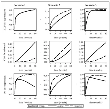
We employ 3 different simulation scenarios shown in Figure 3.1. In scenario 1 the treat-ment group was the same as control in terms of suppression and had much later rebound, thus maintaining suppression much longer than the control group. Under scenario 2, the treat-ment group had faster suppression but also faster rebound. On average, in scenario 2, the treatment group was suppressed longer. In scenario 3, the treatment group suppressed later than in the control group, but maintained suppression longer. Thus, under scenario 3, the treatment group had reduced probability of suppression in the beginning of the observation period which reversed at later times.
We used the Weibull distribution for all time variables in the simulations, due to its flexible shape, with the CDF functionF(t) = 1−exp{−(t
β)
Scenario 1 Scenario 2 Scenario 3
treatment control
Treatment group
0 20 40 60 80
time (weeks) 0.0 0.2 0.4 0.6 0.8 1.0 .
0 20 40 60 80
time (weeks) 0.00 0.05 0.10 0.15 0.20 .
0 20 40 60 80
time (weeks) 0.0 0.1 0.2 0.3 P r. in s up pr es si on
0 20 40 60 80
time (weeks) 0.00 0.05 0.10 0.15 0.20 0.25 0.30 .
0 20 40 60 80
time (weeks) 0.00 0.02 0.04 0.06 0.08 0.10 0.12 .
0 20 40 60 80
time (weeks) 0.00 0.05 0.10 0.15 0.20 0.25 C D F f or r eb ou nd
0 20 40 60 80
time (weeks) 0.0 0.2 0.4 0.6 0.8 1.0 .
0 20 40 60 80
time (weeks) 0.0 0.1 0.2 0.3 .
0 20 40 60 80
time (weeks) 0.0 0.1 0.2 0.3 0.4 C D F f or s up pr es si on
α and β as follows. Scenario 1: the treatment group -αS = 0.2, βS = 4000, αRcond = 4, βcondR = 120, the control group - αS = 0.2, βS = 4000, αRcond = 1.35, βcondR = 64. Scenario 2: the treatment group - αS = 0.4, βS = 800, αR
cond = 1, βcondR = 120, the control group - αS = 0.8, βS = 320, αR
cond = 1, βcondR = 120. Scenario 3: the treatment group - αS = 1, βS = 8, αR
cond = 2, βcondR = 240, the control group - αS = 0.1, βS = 0.0008, αRcond = 1, βcondR = 200. The censoring distribution was the same in both treatment groups and across all scenarios, with αcens = 1.5, βcens = 400. Treatment assigment was generated as a Bernoulli random variable with success probability 0.5. We assessed several sample sizes between 250 and 2000 patients. All simulations were conducted using 1000 samples. For the proposed method, we defined observed data as XiS = min(TiS, Ci), XiR = min(TiR, Ci), δiS = I(XiS = TiS) and
δR
i = I(XiR = TiR). We computed the test statistic WG, with each of the three weight functions described in Section 3.2.
To define virologic failure as in the A5142 trial or for the TLOVR-like endpoint, we first chose a cut-off pointγ0, non-suppression prior to which should be considered a failure. Then,
given the cut-off, we defined the observed data for the composite event in A5142 as:
Xicomp =
(
min(TR
i , Ci), 0< TiS ≤γ0
min(γ0, Ci), γ0 < TiS, and
δcompi =
(
I(Xicomp =TiR), 0< TiS ≤γ0
I(Xicomp =γ0), γ0 < TiS.
Similarly, the data for the TLOVR-like event were defined as:
XiT LOV R =
(
min(TR
i , Ci), 0< TiS ≤γ0
0, γ0 < TiS, and
δT LOV Ri =
(
I(XiT LOV R=TiR), 0< TiS ≤γ0
1, γ0 < TiS.
intent to treat analysis from (Riddler et al., 2008). We looked at a range of possible cut-off points in the definition of composite events for the A5142 and TLOVR endpoints.
The observed type I error rate was close to the nominal level for all three methods, ranging from 0.041 to 0.057 for the proposed endpoint and from 0.040 to 0.060 for A5142 and TLOVR endpoints (not shown in tables). The results for power are summarized in Table 3.1. For the proposed method, the power to reject the null hypothesis was consistent for all scenarios, for all choices of the weight function, and increased with sample size. However, for the A5142 composite endpoint and for TLOVR, the power varied from being higher than that for the proposed method to being almost zero, depending on the scenario and the choice of the cut-off point γ0. For scenario 1, the power for both composite endpoints was much
higher than for the proposed method. For scenario 2, the power for A5142 and TLOVR endpoints was sometimes worse than for the proposed method, depending on the chosen value of the cut-off. The results for scenario 3 are the most interesting. If we look at which treatment arm was selected under scenario 3, for some values ofγ0, the A5142 and TLOVR
analyses always incorrectly selected the control arm. For a large sample size (2000 patients), the null hypothesis was rejected in favor of the wrong treatment group 81% of the time using the A5142 endpoint and 92% of the time using TLOVR. Such a reversal of results happened because both composite endpoints from A5142 and TLOVR re-defined the time of event. For some values of the cut-off γ0 (prior to 12 weeks in the scenario 3), the failures in the
Table 3.1: Simulation results: Power to reject the null hypothesis, and the preferred treatment arm, by value of the cut-off time point for the A5142 and TLOVR endpoints, and by weight fucntion for the proposed method.
Method
Scenario 1 A5142 trial TLOVR Proposed
Cut-off (weeks) Cut-off (weeks) Weight
Sample size 8 16 24 32 40 8 16 24 32 40 unity 1/se cens
125 power 0.58 0.70 0.79 0.86 0.90 0.53 0.57 0.62 0.62 0.64 0.39 0.39 0.36
250 power 0.89 0.95 0.98 0.99 1.00 0.85 0.91 0.92 0.93 0.92 0.67 0.67 0.64
500 power 1.00 1.00 1.00 1.00 1.00 0.99 1.00 1.00 1.00 1.00 0.92 0.92 0.89
1000 power 1.00 1.00 1.00 1.00 1.00 1.00 1.00 1.00 1.00 1.00 0.99 0.99 0.99
Method
Scenario 2 A5142 trial TLOVR Proposed
Cut-off (weeks) Cut-off (weeks) Weight
Sample size 8 16 24 32 40 8 16 24 32 40 unity 1/se cens
125 power 0.30 0.19 0.14 0.11 0.06 0.35 0.26 0.21 0.19 0.15 0.31 0.35 0.32
250 power 0.50 0.36 0.22 0.15 0.10 0.57 0.48 0.33 0.30 0.23 0.57 0.63 0.59
500 power 0.79 0.61 0.43 0.26 0.15 0.85 0.76 0.68 0.55 0.43 0.85 0.89 0.86
1000 power 0.98 0.89 0.68 0.45 0.26 0.99 0.97 0.91 0.82 0.69 0.99 0.99 0.99
Method
Scenario 3 A5142 trial TLOVR Proposed
Cut-off (weeks) Cut-off (weeks) Weight
Sample size 8 10 12 14 16 8 10 12 14 16 unity 1/se cens
Table 3.2: Simulation results: Predicted vs. observed power. Weight
Sample size Unity 1/SE Censoring
Observed Predicted Observed Predicted Observed Predicted
125 0.48 0.50 0.52 0.56 0.44 0.47
250 0.84 0.82 0.87 0.86 0.81 0.78
500 0.99 0.98 0.99 0.99 0.98 0.98
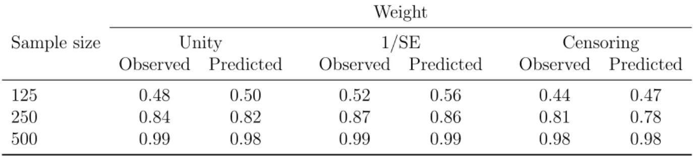
We also conducted a small simulation study to test the sample size computations for the proposed endpoint. We generated 1000 samples from the known distributions under scenario 3 described above, assuming a known effect size. Based on each simulated sample, we esti-mated standard deviations for our test statistics and computed predicted power based on the observed standard deviations and hypothesized effect size (using SAS procedure POWER). Then we compared the average predicted power with the power observed in 1000 simulations. The results summarized in Table 3.2 generally exhibit good agreement between the observed and predicted powers.
3.4 Re-analysis of the A5142 Trial
As an example, we re-analysed the ACTG A5142 trial using the virologic failure endpoint from A5142 and the proposed method. The A5142 trial included 753 patients whose baseline viral load was at least 2000 copies/ml. Patients were randomized to one of the three treat-ment arms, efavirenz plus two NRTIs (efavirenz group), lopinavir–ritonavir plus two NRTIs (lopinavir–ritonavir group), or lopinavir-ritonavir plus efavirenz (NRTI-sparing arm). The median follow-up was 112 weeks, with the longest follow-up time being 157 weeks.
The definition of a virologic failure for A5142 ((Riddler et al., 2008), p.2097) was lack of confirmed viral load suppression below 200 copies/ml or by log10 by 8 weeks; or lack of
Pr
ob
ab
il
it
y
of
N
o
V
ir
ol
og
ic
F
ai
lu
re
0.5 0.6 0.7 0.8 0.9 1.0
Weeks from randomization
0 10 20 30 40 50 60 70 80 90 100 110 120 130 140 150 160
Treatment Group: NRTI-sparing
Lopinavir-ritonavir Efavirenz
Pr
ob
ab
il
it
y
to
B
e
in
S
up
pr
es
si
on
0.0 0.2 0.4 0.6 0.8 1.0
Weeks from randomization
0 10 20 30 40 50 60 70 80 90 100 110 120 130 140 150 160
Treatment Group: NRTI-sparing
Lopinavir-ritonavir Efavirenz
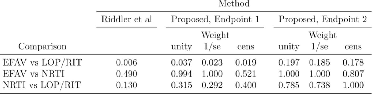
Table 3.3: P-values comparing between treatment groups in the A5142 trial, original analysis vs. proposed method. Endpoint 1: single threshold of 200 copies/ml in the definitions of suppression and rebound. Endpoint 2: different definitions for early and late suppression and rebound. P-values adjusted for multiple comparisons using the Bonferroni correction.
Method
Riddler et al Proposed, Endpoint 1 Proposed, Endpoint 2
Weight Weight
Comparison unity 1/se cens unity 1/se cens
EFAV vs LOP/RIT 0.006 0.037 0.023 0.019 0.197 0.185 0.178
EFAV vs NRTI 0.490 0.994 1.000 0.521 1.000 1.000 0.807
NRTI vs LOP/RIT 0.130 0.315 0.292 0.400 0.785 0.738 1.000
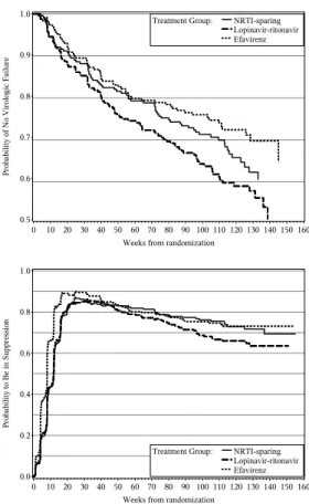
For the proposed approach, we defined two separate events, viral suppression and viral rebound. We defined viral suppression as viral load being reduced to < 200 copies/ml for two consecutive measurements 4 weeks or less apart. We defined viral rebound as viral load being ≥ 200 copies/ml at two consecutive measurements 4 or less weeks apart. We had 667 patients in all treatment groups whose viral load was suppressed, and 129 patients who experienced viral rebound. A plot of the estimated probability of being suppressed, over time from randomization, by treatment group, is displayed on the bottom panel of Figure 3.2.
We defined early viral suppression and viral rebound prior to 32 weeks as was done in the A5142 trial. Under this definition, the number of patients in all treatment groups who experienced viral suppression was 691, and who experienced viral rebound was 183. The results of this supplementary analysis are also summarized in Table 3.3 as endpoint 2 and are not statistically significant at 0.05 level, though the direction of the differences remained the same.
We also performed sensitivity analysis to assess how much the results of the A5142 trial depended on the choice of cut-off time of 8 weeks for early rebound and 32 weeks for late rebound. Judging by the plot of the probability to be in suppression by treatment group, we did not expect inference to change when we varied the cut-off times for early and late viral rebound. This is because the best treatment group was uniformly better than the second best treatment group both in terms of viral suppression and viral rebound, with the same ordering holding for the second and third best treatment groups. We re-defined virologic failure using cutoffs ranging from 5 to 15 weeks for early rebound and from 25 to 40 weeks for late rebound. The results confirmed our expectations: the p-values for comparison of the efavirenz and lopinavir-ritonavir groups remained significant and ranged from 0.0107 to 0.0306 (after a Bonferroni correction), all other comparisons were still not statistically significant, and all the differences between the groups were in the same direction.
In summary, certain advantages of the proposed endpoint can be clearly seen in Figure 3.2, where the time-specific treatment differences are cleanly summarized via the probability of being in suppression. The efavrienz group suppresses most rapidly and with higher prob-ability and the suppression is maintained as effectively as in the NRTI-sparing arm. The NRTI-sparing arm has comparable early suppression to that in the lopinavir group, but with superior long term maintenance. Such information is not as readily gleaned from the plot of the survival curves for the A5142 composite endpoint.
3.5 Discussion
DeGruttola (DeGruttola et al., 1998) were the first to discuss the use of HIV-1 RNA viral load as an outcome measure in HIV trials, both as a repeatedly-assessed continuous biomarker and as an indicator of treatment (virologic) failure. (Gilbert et al., 2000) expand on the discussion of virologic failure and consider several competing definitions. (Ribaudo et al., 2006) discussed design issues in HIV trials, concentrating the discussion of endpoints on further refinements in virologic failure. To the best of our knowledge, no one has previously suggested the combined endpoint we propose here.
HIV research that combines time to viral suppression and time to viral rebound into a single measure, the probability of being suppressed over time. As demonstrated in the A5142 data analysis, this quantity precisely captures the interplay of suppression and rebound, yielding a simple graphical representation of early and late suppression dynamics which may be preferable to that for the existing composite endpoints. The integrated probability of suppression can easily be adapted by choice of the weight function to target specific time periods of interest. Employing unity weight provides a particularly attractive summary which may be interpreted as the average number of weeks suppressed over the time period of interest. If there is scientific justification to disregard a portion of the follow-up period, the weights function can be set to zero for those times points.