Quantum Random Walk Search and Grover's Algorithm - An Introduction and Neutral-Atom Approach

(1)

Quantum Random Walk Search and Grover’s Algorithm

-An Introduction and Neutral-Atom Approach

A Senior Project

presented to

the Faculty of the Physics Department

California Polytechnic State University, San Luis Obispo

In Partial Fulfillment

of the Requirements for the Degree

Bachelor of Science

Computer Engineering

by

Anna Maria Houk

(2)

1 Introduction

Modern computing has become increasingly powerful, but there are still hard limits on the the time com-plexity and problems that can be solved. Some of these limits can however, be breached by quantum computers, which use quantum mechanical properties to encode information into quantum particles re-ferred to as qubits and perform computations. In the sub-field of quantum algorithms, physicists and computer scientist take classical computing algorithms and principles and see if there is a more efficient or faster approach implementable on a quantum computer, i.e. a ”quantum advantage”.

In classical computing, random walks are defined as a sequence of random steps on a mathematical space and are used in computer science and other fields to model natural phenomena. Random walks are a special case of a stochastic model (i.e. a random mathematical process) known as Markov chains, which is a process during which predictions can be made at any state in the process without knowledge of the past states with the same accuracy [1]. There are already many classical applications of random walks in fields such as reinforcement learning, random number generation, and thermodynamics to name a few, so it is a natural question of interest to if there is a similar usefulness for random walks implemented with quantum computers. Exploration of continuous and discrete-time quantum random walks and classical random walks with discrete state-space have shown that there is a quantum advantage and significant differences in the behavior between the classical and quantum random walks [2] [3].

In this paper we will begin by taking classical examples of random walks and move them into the quantum computing paradigm, as well as introduce a popular quantum search algorithm called Grover’s search. There are currently many methods being explored for creating quantum computers and qubits, but in Section 3, we will look at using neutral-atom (also known as cold-atom) quantum computing to physically implement the random walks and Grover’s algorithm. Lastly, using similar principles to Grover’s, we will explore a possible application of quantum random walks as a search algorithm.

2 Background

2.1 Discrete Quantum Random Walks

(4)

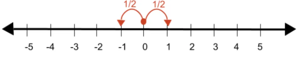
number line. At each step in the walk there is an equal probability that the next position will be either the previous position or the next integer on the number line and transition probabilities are only dependent on the current step. If the probability of ending up at each position is looked at aftertsteps, it will approach a Gaussian distribution at a large number of iterationsT, centered around zero (the initial position) and a variance ofδ2 =Ti.e. an average distance√T from the initial position [3].

Figure 1: A one-dimensional random walk

Taking the number-line and coin flip random walk model to the quantum paradigm, the number-line can be expressed as a one-dimensional space being traversed by a spin-1₂ particle [2]. The position of the particle is the substitute for the position of the number-line and the spin of the particle takes the place of the coin. Study of the mathematics of quantum mechanics shows that the walk of the particle is described by the unitary operator written in such a way to separate the spin and position state spaces:

U =e−2iSz⊗P l ₍₁₎

More information about this operator can be found in much greater depth in [4], but only a surface-level understanding is needed for this paper, specifically the separability of the spin and position state spaces and how they are utilized in a random walk. Above,Pis the momentum operator andlis the constant step length with each iteration to create a discrete state-space. Sz is the operator that represents the z-component of the spin of the particle and is written as:

Sz =

1 2

1 0

0 −1

= 1

2(|↑i h↑| − |↓i h↓|) (2)

The operator is applied to the particle described by the wave function in the initial state,

(5)

is in equal superposition for the spin (α=β= √1

2). Applying the unitary operator results in:

U|ψ0i=α|↑i |ψx0−li+β|↓i)|ψx0+li (3)

|↓i, much like flipping a coin has an equal chance of landing heads or tails. In quantum computing the state-space, or registers, of a computer are described as a Hilbert space. Therefore, we will rewrite the quantum walk model in terms of the ”registers” of a quantum machine in order to use the quantum random walk computationally.

Take the discrete space travelled by the particle to be of length N. Each position will be a basis state and the last position,|N−1i, leads to position|0i, so the space is essentially a circle. The Hilbert space that the discrete quantum walk exists in can be again be separated into the spin and state space:

H=Hc⊗Hp (4)

WhereHp is the size N positional Hilbert space, Hp = {|ii : i = 0,1,2, ..., N −1}, andHcis the coin space consisting of the two spin states,Hc ={|↑i,|↓i}. With these definitions, the operation in Equation (1), which is responsible for the direction of movement of the particle, can be written as a new unitary operator:

S =|↑i h↑| ⊗

N−1

X

i=0

|i+ 1i hi|+|↓i h↓| ⊗

N−1

X

i=0

|i−1i hi| (5)

Now a mechanism is needed to ”flip the coin”. A common choice is to use a single-qubit gate referred to a Hadamard gate

H= √1

2

1 1

1 −1

= √1

2(|↑i h↑|+|↑i h↓|+|↓i h↑| − |↓i h↓|) (6)

(6)

a coin is the unitary

Uwalk=S·(H⊗I) (7)

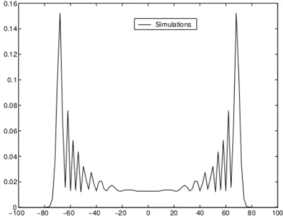
IfUwalkiterates T times, as done with the classical model, the behavior differs immensely. The resulting distribution does not come to approximate a Gaussian distribution and instead has a close to uniform spread over the interval[−√T

2, T

√

2]and has a variance ofδ

2 ₌ _T2 _{i.e. an average distance T from the} initial position. Figure 2 is depicts the probability distribution of a 100-step walk from [2].

Figure 2: The probability distribution of a quantum walk using a Hadamard gate as the coin

2.2 Continuous Quantum Random Walks

(7)

each position on the number line, the probability of a transition is 1₂ for j = i±1 and 0 for all other scenarios. The transition matrix M for jumping on a number line (that circles around) of five positions is as follows:

M = 1 2



    

0 1 0 0 1

1 0 1 0 0

0 1 0 1 0

0 0 1 0 1

1 0 0 1 0



    

(8)

Written generally for n-number of positions on a number line:

Mij =

(₁

2, j=i±1.

0, j6=i±1. (9)

While the transition matrix stays the same no matter what point in time, the probability of ending up at positionjfrom positioniafter T will evolve at each step, but given the independence of each step, the probability at each time-step,pt, will only depend on the previous move. This means that the probability at each step is

pt+1=M pt. (10)

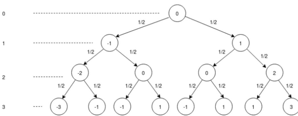
The evolution of each step and the number of possible ending positions oftiterations can be described as a decision tree, shown visually in Figure 3. Each level of the tree is an iteration of the walk and each node the position on the number-line with each branch stemming out of a node being a possible next step from that node. Since we know all possible outcomes that could happen from the starting node after T iterations of the walk, the walk along the number-line can also be thought of as a traversal through its decision tree. Now, it appears that this walk is still operating discretely, so in order to turn this into a continuous walk we assume that a transition could occur at anytime in the walk at a rate ofγ, which is a fixed constant rate. The iterations in the walk are still measured in discrete time units, but the jump to the next position on the number line occurs with a probabilityγwith each passing unit of time. Thus, the entire walk is conducted in theHp state space and a new continuous transition matrix H can be written:

Hij =

  

 

−γ, j=i±1

0, j6=i±1andi6=j 1

2γ, i=j

(11)

(8)

Figure 3: The decision tree to T=4 iterations of walking on a number-line

new continuous probability of being at a a positioniat some timetis described by: dpi(t)

dt =− X

j

Hijpj(t) (12)

Solving with an assumption of an initial position of 0, the probability at timetbecomes:

p(t) =e−Htp(0) (13)

To move the continuous walk into the quantum space, a quantum operator can be constructed using the continuous transition matrix H:

Uwalk(t) =e−iHt (14)

From [7], at anytime t in the walk the state of the walk will be a superposition of the basis states, i.e. the possible positions on our number-line or the nodes reachable from our place on the decision tree, which all exists in our Hilbert spaceHp, as defined in the discrete walk section. The results of the continuous walk show the same quantum advantage as the discrete quantum walk, even though the mechanics of how the walks operate are not the same. Currently there is little known about the relationship between the discrete and continuous quantum walks and is an open research area.

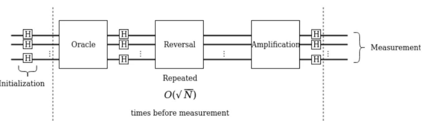
2.3 Grover’s Search

(9)

Figure 4: A high-level representation of the key components of Grover’s algorithm. The algorithm is run

p

(N)times on the input, where N is the number of qubits of the input.

2.3.1 The Oracle Circuit

The oracle portion of the circuit is dependent on the application of the algorithm, so it is left as a ”black-box” in its general form. The operation of the oracle is to take the search space (i.e. the superposition of all possible states) as an input and mark the item that is being searched for (i.e. one of the states in the input with a negative sign). Figure 5 shows some examples of oracle circuits for an N=2 circuit.

(a) Oracle marks state of|00i (b) Oracle marks state of|01i

(c) Oracle marks state of|10i (d) Oracle marks state of|11i

(10)

The operation of the oracle [9] can be generally described as:

|xi |qi → |xi |q⊕f(x)i (15)

Where x is the element being evaluated and q is a single qubit that will flip if f(x) = 1, where f(x) is a function that determines whether x is what we’re searching for. q is set to be in superposition so that the oracle has the following behavior:

|xi(|0i − |√ 1i

2 )→

(

|xi(|1i−|√ 0i

2 ), iff(x) = 1.

|xi(|0i−|√ 1i

2 ), iff(x) = 0.

(16)

This can be rewritten as a sign-flip controlled by the result of f(x) as so:

|xi(|0i − |√ 1i

2 )→ |xi(−1)

f(x)₍|0i − |_√ 1i

2 ) (17)

This shows that solutions to the oracle will be marked negatively, which can cleverly be used later in the amplification circuit. Since the value of q does not change other than in sign, the behavior of the oracle can be most simply written as:

|xi → |xi(−1)f(x) (18)

2.3.2 Example of the Oracle

An example of applying the oracle from Figure 5 (c) to the input|xiis shown below. First lets define the gates used in the oracle:

X =

0 1 1 0

I ⊗X=



  

0 1 0 0

1 0 0 0

0 0 0 1

0 0 1 0

    CZ=    

1 0 0 0

0 1 0 0

0 0 1 0

0 0 0 −1



  

(19)

The X-gate is only applied to the second qubit, so to get a two-qubit definition we take the tensor prod-uct of the Identity with the X-gate, as the Identity will change the values of the first qubit. The CZ, orcontrolled-Z, gate is the definition of the two-qubit gate labeled ”Z” in Figure 5 (c). We can now construct:

ˆ

f(x) =I⊗X·CZ·I⊗X

=



  

0 1 0 0

1 0 0 0

0 0 0 1

0 0 1 0

       

1 0 0 0

0 1 0 0

0 0 1 0

0 0 0 −1

       

0 1 0 0

1 0 0 0

0 0 0 1

0 0 1 0



  

(11)

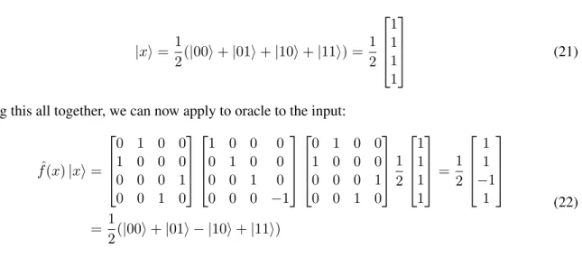
The input|xiwill start in an equal superposition:

|xi= 1

2(|00i+|01i+|10i+|11i) = 1 2     1 1 1 1     (21)

Putting this all together, we can now apply to oracle to the input:

ˆ

f(x)|xi=



  

0 1 0 0

1 0 0 0

0 0 0 1

0 0 1 0

       

1 0 0 0

0 1 0 0

0 0 1 0

0 0 0 −1

       

0 1 0 0

1 0 0 0

0 0 0 1

0 0 1 0

    1 2     1 1 1 1     = 1 2     1 1 −1 1     = 1

2(|00i+|01i − |10i+|11i)

(22)

After applying the oracle, the state|10inow has a negative amplitude.

2.3.3 The Amplification Circuit

Taking off from where the oracle has left our qubits, we will have the solution ”marked” with a negative amplitude. Simply having a negative amplitude will not help when it comes to taking a measurement, as while the reflection does lower the average amplitude of x, it is not significant enough to detect the solution in a measurement. An additional reflection, however, can be performed to boost the amplitude of our negatively-marked solution(s) [9], moving the state closer to that of the solution state.

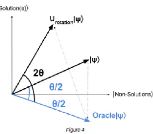
Figure 6: The ”amplification” or “rotation” circuit for a 2-qubit system.

(12)

Figure 7: A visual representation of the reflections performed on|ψi, the superposition of all states, by the oracle and amplification circuits on a plane defined by the superposition of all solution states and the superposition of all non-solution states. Aθshift is applied with each iteration of Grover’s algorithm.

phase shift:

|xi → −(−1)δx0_|_x_i ₍₂₃₎

Whereδx0represents a conditional component that applies a negative sign to all states except|0i. Lastly, apply another Hadamard gate to x.

A more technical definition of this rotation can be summed up by defining the following operator as the identity subtracted from twice the projector onto|ψi, the equal superposition of all states.

Urotation= 2|ψi hψ| −I (24)

2.3.4 Example of the Amplification Operation

Going back to the state of the input register|xifrom the oracle in Equation (22), we will now apply the amplification operation to|xi. Since this example is a two-qubit system, the time-complexity isO(√2). Only one iteration is needed to find the target state. As the Hadamard and X gates are applied to both qubits, the matrices are:

H⊗H= 1 2



  

1 1 1 1

1 −1 1 −1

1 1 −1 −1

1 −1 −1 1



  

X⊗X =



  

0 0 0 1

0 0 1 0

0 1 0 0

1 0 0 0



  

(13)

The two-qubit gate in Figure 6 is a cNot, orcontrolled-not, gate and will flip the value of the second qubit if the value of the first qubit is in the excited state. However, the second qubit also has a Hadamard applied before and after the cNot gate, which combined becomes:

I⊗H= √1

2



  

1 1 0 0

1 −1 0 0

0 0 1 1

0 0 1 −1



  

cN OT =



  

1 0 0 0

0 1 0 0

0 0 0 1

0 0 1 0



  

(26)

(I⊗H)·CN OT ·(I⊗H) =



  

1 0 0 0

0 1 0 0

0 0 1 0

0 0 0 −1



  

(27)

Which is the theCZ gate from Equation (19). Putting all the pieces together to construct the amplifica-tion operator:

Urotation= (H⊗H)·(X⊗X)·cN ot·(X⊗X)·(H⊗H)

= 1 2    

1 1 1 1

1 −1 1 −1

1 1 −1 −1

1 −1 −1 1

       

0 0 0 1

0 0 1 0

0 1 0 0

1 0 0 0

       

1 0 0 0

0 1 0 0

0 0 1 0

0 0 0 −1

       

0 0 0 1

0 0 1 0

0 1 0 0

1 0 0 0

    1 2    

1 1 1 1

1 −1 1 −1

1 1 −1 −1

1 −1 −1 1



  

(28) Applying the operator to the input:

Urotation|xi

= 1 2    

1 1 1 1

1 −1 1 −1

1 1 −1 −1

1 −1 −1 1

       

0 0 0 1

0 0 1 0

0 1 0 0

1 0 0 0

       

1 0 0 0

0 1 0 0

0 0 1 0

0 0 0 −1

       

0 0 0 1

0 0 1 0

0 1 0 0

1 0 0 0

    1 2    

1 1 1 1

1 −1 1 −1

1 1 −1 −1

1 −1 −1 1

    1 2     1 1 −1 1     = 1 8     0 0 8 0    

=|10i

(14)

3 Implementation

3.1 Neutral-Atom Quantum Computing

In neutral atom quantum computing the qubits are represented by contained and addressable atoms. This is accomplished by first cooling and trapping neutral atoms with lasers and magnetic fields inside a magneto-optical trap (MOT). Once they have been trapped in the MOT, the cold atoms are transferred to a light pattern where they can be held as an array of individually addressable atoms. The result of a narrow-band laser excitation of atoms can be found starting from the time-dependent Schr¨odinger equation representing an atom in a radiation field and then making approximations to constrain ourselves to a Rabi two-level problem [11], a solution of just two states. We refer to these two states as the ground state (i.e.|0i), denoted asgbelow, and excited state (i.e. |1i), denoted asebelow, the equations for the probability amplitudes of these two states are found to be:

    

   

cg(t) = (cos(

Ω0t

2 )−i

δ

Ω0sin( Ω0t

2 ))e

+iδt/2

ce(t) =−i

Ω Ω0sin(

Ω0t

2 )))e −iδt/2

(29)

Where|cg(t)|2 and|ce(t)|2 give the respective probability of finding the atom in that state, with this probability oscillating at an angular frequency ofΩ0 ≡p

(Ω2+δ2). The angular frequency at which the probability oscillates is dependent onΩ≡ −eEo

~

(15)

Figure 8: Illustration from [11] of the probability of an atom to be in the excited state forΩ =γin time units of1_γ at different laser detunings.

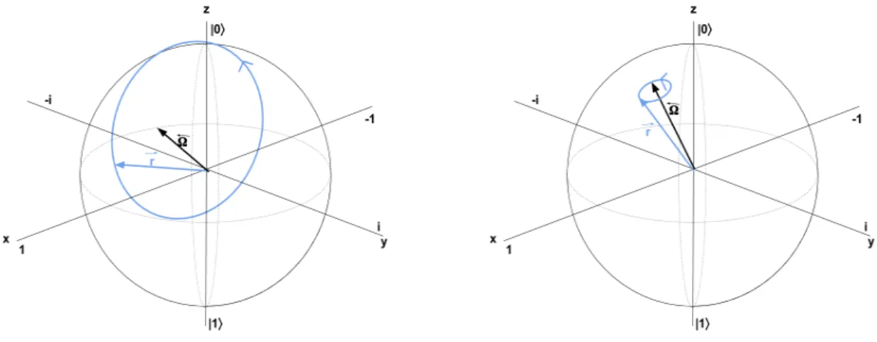
3.1.1 Building Quantum Gates

(16)

(a) Near zero detuning for Hadamard gate (b) Large detuning for an X-gate

Figure 9: Single qubit gates on the Bloch sphere

For a two-qubit gate, there needs to be an interaction between the control and target qubits. In [12] a neutral-atom approach to a cNOT gate is built using the Rydberg blockade to block the excitation of the target atom if the control is in the excited state. Figure 10 depicts the order and phaseamountof the Rabi oscillation of applied laser pulses for the cNOT gate. A Hadamard rotation (aπ₂ phase to the wave function) is applied to the target before and after the cPHASE operation(pulses 2, 3, 4). If the control is|0i, the target is uninhibited from transitioning to the basis or excited state. If the control is|1i, the control is excited into the Rydberg level which prevents pulse 3 from having any effect on the target atom because of the Rydberg blockade.

(17)

These gates are the all the components needed to implement Grover’s search algorithm. In summary, the series of gates depicted in Section 2.3 that make-up Grover’s are an arrangement of a series of laser pulses applied to lattice sites.

3.1.2 Discrete Walk with Neutral Atoms

The discrete quantum walk of section (2.2) using a Hadamard coin has already been physically imple-mented [13]. In this section we will cover the physical set-up for the n-step walk using the definitions of S and H from equations (5) and (6):

|ψni= (SH)n|ψ0i (30)

The system will be made up of two, one-dimensional lattices, each for trapping a different of the basis states of a neutral atom. The lattices are identical and made up of optical potentials of perioddthat form through counter-propagating harmonic waves with electric fields forming an angle2θ. The lattices are manipulated by changing the angleθ, which causes the left and right circular polarized components of the standing wave that form the total electric field to shift [13]. Lattice0, which holds atoms in the basis state|↑iand will move with constant velocityv0 =−vto the left while lattice1 holds atoms in the basis state|↓iand will move with constant velocityv0 =vto the right.

The walk will start by placing a single neutral atom prepared in state √1

2(|0i+i|1i)in the lattice0 at the minimum of a potential well which we will refer to asx0at timet0. The Hadamard gate, as described in Section 3.1.1, will then be applied periodically att= nd_v to all trap locations in the lattice. The atom will move with constant velocity with the lattice it is trapped in determining the direction of travel:

x(t) =

(

x0−vt,(i.e. left) if|↑i x0+vt,(i.e. right) if|↓i

(31)

(18)

resulting from the aforementioned applied pulse. Running this procedure multiple times will result in the ending location of the particle to match the distribution shown in Figure 2, the expected distribution for a symmetric discrete quantum one-dimensional random walk.

3.1.3 Continuous Walk with Neutral Atoms

An implementation of a continuous quantum random walk in one dimension has been proposed using Rydberg atoms [14] but yet to be done experimentally. Using the blockade mechanisms and strong interactions of Rydberg atoms, [14] fills the sites of an optical lattice with neutral atoms and then promotes one atom in each trap location to higher energy levels to perform the continuous walk.

The energy states of atoms greatly effect the interaction energy between two atoms. Atoms excited to annpenergy level will have very strong interactions with other atoms in that state. Atoms in anns energy level will have weak interactions with atomsnpstate due to the large difference in energy as well as with othernsenergy atoms. As a result, Rydberg atoms, which have a very large radii and strong dipole moments, will lead to a blockade mechanism taking place. The blockade means that only one atom can be excited into a Rydberg state due to large shifts in energy levels and other atoms interacting with a Rydberg atom will be prevented from being promoted to a high-energy state. Using this property, [14] studies the diffusion of an excited state among many sites in a lower energy state as a way to perform a continuous walk along an optical lattice.

(19)

As seen in Figure 11, instead of trapping a single atom as done for the discrete walk in [13], a cluster of atoms are trapped at trap locations about 25µm apart, in order to facilitate easy addressing and detection at each site as well as site separation having an effect on the timescale of how quickly iterations occur [14]. For N-1 of the sites, one atom in each cluster will be promoted to a Rydberg statens. The last remaining site will be promoted to a Rydberg statenpand will be considered thex0 location of the walk. Thenpexcitation will rapidly transfer from trap site to trap site by a phenomenon called resonant transfer. One step (i.e. one hop along our line) will occur within the time increment that is dependant on the dipole interaction energy between the atoms,τhop∼ _4V_dipoleh withVdipole∼ n

4

R3, n being the principle quantum number and R being the distance of the inter-atomic separations. Using the set-up proposed, the time between hops will be,τhop ∼ h

4n4 R3

= h

4(70)4 (25)3

giving usτhop ∼170ns. Waiting for a period of time equal to n iterations passing, the position of thenpexcited state is measured, completing the walk. Performing many repetitions of this the walk procedure will produce a ending-position distribution of the walk matching Figure 2.

4 The Quantum Random Walk Search

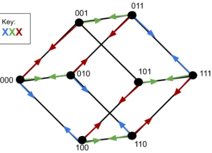
Algorithms based on quantum random walks are still in infancy, but a search algorithm has been pro-posed [15] using a discrete quantum random walk along a hypercube. The algorithmic steps and unitary operator of the quantum random walk search appear quite similar to Grover’s search algorithms. The unique properties of the random walk may provide an ease in implementation over other quantum search algorithms, but unfortunately adds complexity to its analysis.

(20)

Figure 12: The position space for a walk along a hypercube when n = 3. The graph vertexes are color-coded by direction, i.e. which bit in the binary string is flipped in the transition between nodes

next step, making the total Hilbert space of the search:

H =Hn⊗HN (32)

Like Grover’s search, the quantum walk search operator can be broken up into two main components, the shift-operator and the coin-flip. The shift operator creates a superposition of all possible position state transitions and can be described as the following mapping:

S=

n−1

X

d=0 N−1

X

x=0

|d, x⊗edi hd, x| (33)

(21)

S =

2

X

d=0 7

X

x=0

|d, x⊗edi hd, x|

=|0,000⊕e0i h0,000|+|0,001⊕e0i h0,001|+...+|0,111⊕e0i h0,111|

+|1,000⊕e1i h0,000|+|1,001⊕e1i h1,001|+...+|1,111⊕e1i h1,111|

+|2,000⊕e2i h2,000|+|2,001⊕e2i h2,001|+...+|2,111⊕e2i h2,111|

=|0,000⊕001i h0,000|+|0,001⊕001i h0,001|+...+|0,111⊕001i h0,111|

+|1,000⊕010i h0,000|+|1,001⊕010i h1,001|+...+|1,111⊕010i h1,111|

+|2,000⊕100i h2,000|+|2,001⊕100i h2,001|+...+|2,111⊕100i h2,111|

=|0,001i h0,000|+|0,000i h0,001|+...+|0,110i h0,111|

+|1,010i h0,000|+|1,011i h1,001|+...+|1,101i h1,111|

+|2,100i h2,000|+|2,101i h2,001|+...+|2,011i h2,111|

Now, a coin operator must be chosen to act onHc. A common coin to use is the rotation operator from Equation (20) that is commonly referred to as ”Grover’s diffusion operator”. We will refer to the operator from (20) as the following to be clear on the space that the operator is applied to:

G=Urotation = 2|ψci hψc| −I (34)

Where|ψciis the superposition over all n directions of walking on the hypercube. The Grover coin is a useful coin as it is the operator the farthest away from the identity operator, which makes it efficient in mixing, which means to reach a stationary distribution, over states regardless of the initial position of the walk.

In order to construct a search algorithm, the operation in the coin will be used like the Oracle in Grover’s, to ”mark” the node that we are searching for. However, only using the Grover diffusion operator as the coin/oracle in the quantum walk such that the quantum walk operator is defined as:

(22)

However, applying this operator will not change the state of the system if starting from a superposition of the entire Hilbert space. Instead of just applying a negative phase to the node that is being searched for, the oracle/coin operator for the quantum random walk search will apply one coin,C, which [15] chooses to beC=−Ifor simplicity in analysis, to the the target node and the Grover diffusion operator, Gto all of the other nodes, creating the coin operator:

C0 =G⊗I+ (C−G)⊗ |xtargeti hxtarget| (36)

Using this hybrid coin, the unitary evolution operatorU0is: U0 =S·C0

=S·(G⊗I+ (C−G)⊗ |xtargeti hxtarget|)

=U −2S·(|ψci hψc| ⊗ |xtargeti hxtarget|)

(37)

Analysis in [15] shows that the perturbation of this operator results in the quantum random walk search algorithm. Now that all parts of the perturbed unitary operator used in this search algorithm have been defined, the steps for its implementation are the following:

1. Apply a Hadamard gate to the all qubits to initialize the entire Hilbert space to be in an equal super position,|ψ0i

2. Apply the quantum walk search unitary operator,U0, to|ψ0i 3. Repeat step 2O(√N)times

4. Measure the state of the system

4.1 Similarities to Grover

(23)

Figure 13: The quantum random walk high-level circuit

1. The random walk search is not an exact mapping onto a two-dimensional subspace

2. The subspace contained by the walk is spanned by (1) a superposition of all states, and (2) a close approximation to the target state, unlike Grover’s which is spanned by (1) all non-target states and (2) the target state(s)

3. The final state contains small contributions from its neighbor nodes, unlike Grover’s in which the final state is ends up as purely the target state

These differences are yet to be found as advantages or disadvantages, and will be open questions until more work is done experimenting with these algorithms on different quantum hardware.

4.2 The Eigenvectors and Sub-Space

(24)

Figure 14: The n=3 walk reduced to an unbalanced walk on a line. The nodes of the walk are now the the possible Hamming weights of an n=3 graph rather than n-bit binary strings.

4.2.1 The Approximate Eigenvectors of U’

We begin with defining two approximate eigenvectors ofU0,|ψ0i, the superposition over all states and transitions, and|ψ1i, an approximation of the target state. For the examples that follow, we will assume the target statextarget = 0. The definition of|ψ0iis as follows1:

|ψ0i=

1

√

N |R,0i+

1

√

N |L, ni+ n−1

X

x=1

(

s

n−1 x−1

N |L, xi+ s

n−1 x

N |R, xi) (38) Notice that now the superposition over the states is not an equal superposition anymore, with lower probabilities on the farthest left and farthest right node. Expandingψ0for then= 3walk becomes:

|ψ0i=

1

√

8|R,0i+ 1

√

8|L,3i+

2 X x=1 ( s 2 x−1

8 |L, xi+

s

2 x

8 |R, xi) = √1

8|R,0i+ 1

√

8|L,3i+ 1

√

8|L,1i+ 1

2|R,1i+ 1

2|L,2i+ 1

√

8|R,2i

Note that now x represents the Hamming weight of a position along the line rather than the individual bit sequence of each node due to the collapse of the reduction in dimensions.

1

In case it is unfamiliar, the mathematical symbol n_x

is the binomial function and is defined as n_x

(25)

Now to find the second approximate eigenvector letψ1be defined as2:

|ψ1i=

1

c bn

2−1c X

x=0

(

s

1

n−1 x

|R, xi − s

1

n−1 x

|L, x+ 1i) (39)

Wherec=

r Pbn

2−1c

x=0 (

1

(n−1

x )

, is a normalization constant. Expandingψ1 for then= 3walk becomes:

|ψ1i= 0

X

x=0

(

s

1

2 x

|R, xi − s

1

2 x

|L, x+ 1i), c= 1

= √1

2|R,0i − 1

√

2|L,1i

This vector includes all states in the target position as well as states with a non-zero probability of transitioning to the target state.

4.2.2 The Sub-Space of U’

As mentioned previously, the spanned space of the walk is contained within a complex conjugate pair of eigenvectors ofU0we will call|ω0+iand|ω0−i. A spectral analysis onU0(see Appendix A), confirms

2

(26)

that there are only two eigenvalues with a real component greater than1− 2

3n. These eigenvectors can be well approximated by|ψ0iand|ψ1i(proof in [15]) as the following linear combinations:

|ω0+i ≈

1

√

2(|ψ0i+i|ψ1i)

|ω0−i ≈ 1

√

2(|ψ0i −i|ψ1i)

(40)

√

N) number of times, |ψ0i will rotate sufficiently close to|ψ1ito successfully measure|xtargeti. As with all quantum algorithms, a single run will have error, but it can be made arbitrarily small without increasing complexity by repeating the algorithm a fixed number of times.

5 Conclusions

(27)

6 Appendix A

The following calculations were done following the results of [15].

Figure 16: The spectral analysis of an n = 3 search. The red points are the eigenvalues ofU0 and the blue is are the eigenvalues ofU. The arc spans the1−_3n2 area the eigenvalues of|ω0+iand|ω0−icould

(28)

The values of the eigenvalues and corresponding eigenvectors closest to the real axis for the n = 3 walk are:

eigenvalue0 = 0.8819171 + 0.47140452i eigenvector1 = 0.8819171−0.47140452i

eigenvector0 = eigenvector1 =

                                            

2.67261242×10−01 +0.0i

−2.35702260×1001 ₊₁_._25988158_×₁₀01_i

1.17851130×1001 +1.25988158×1001i −4.45435403×1002 +1.66666667×1001i

1.17851130×1001 ₊₁_._25988158_×₁₀01_i

−4.45435403×1002 +1.66666667×1001i

8.90870806×1002 +1.66666667×1001i

2.15952654×1016 +1.88982237×1001i

2.67261242×1001 −8.34332948×1017i

1.17851130×1001 +1.25988158×1001i −2.35702260×1001 +1.25988158×1001i −4.45435403×1002 +1.66666667×1001i

1.17851130×1001 +1.25988158×1001i

8.90870806×1002 +1.66666667×1001i −4.45435403×1002 +1.66666667×1001i

8.75973249×1017 +1.88982237×10−01i

2.67261242×1001 −6.12696729×10−17i

1.17851130×1001 +1.25988158×10−01i

8.90870806×1002 +1.66666667×10−01i −2.35702260×1001 +1.25988158×10−01i −4.45435403×1002 +1.66666667×10−01i −4.45435403×1002 +1.66666667×10−01i −5.00035475×1017 +1.88982237×10−01i                                                                                          

2.67261242×1001 −0.0i

−2.35702260×1001 ₋₁_._25988158_×₁₀01_i

1.17851130×1001 −1.25988158×1001i −4.45435403×1002 −1.66666667×1001i

1.17851130×1001 ₋₁_._25988158_×₁₀01_i

−4.45435403×1002 −1.66666667×1001i

8.90870806×1002 −1.66666667×1001i

2.15952654×1016 −1.88982237×1001i

2.67261242×1001 +8.34332948×1017i

1.17851130×1001 −1.25988158×1001i −2.35702260×1001 −1.25988158×1001i −4.45435403×1002 −1.66666667×1001i

1.17851130×1001 −1.25988158×1001i

8.90870806×1002 −1.66666667×1001i −4.45435403×1002 −1.66666667×1001i

8.75973249×1017 −1.88982237×1001i

2.67261242×1001 +6.12696729×1017i

1.17851130×1001 −1.25988158×1001i

8.90870806×1002 −1.66666667×1001i −2.35702260×1001 −1.25988158×1001i −4.45435403×1002 −1.66666667×1001i −4.45435403×1002 −1.66666667×1001i −5.00035475×1017 −1.88982237×100i

                                            

(29)

import numpy as np

import matplotlib as mpl

import matplotlib.pyplot as plt

#set the number of dimensions

n = 3

N = pow(2, n)

np.set_printoptions(linewidth=np.inf)

psi_proj = (1/n)*np.matrix(np.ones((n, n))) #superposition of coin space

Co = 2*psi_proj - np.matrix(np.identity(n))

print("Co:\n", n*Co, "\n")#factor out normalization for ease of reading

C = np.matrix(np.kron(Co, np.identity(N))) print("C:\n", n*C, "\n")

S = np.matrix(np.zeros((n*N, n*N))) d = 0

for i in range(0, n):

for x in range(0, N):

ed = d + pow(2, i) S[xˆed, x+d] = 1 S[x+d, xˆed] = 1 d += N

print("S:\n", S, "\n")

U = S*C

print("U:\n", n*U, "\n")

zero_proj = np.matrix(np.zeros((N, N))) zero_proj[0,0] = 1

#the qrw unitary operator

U_ = U - 2*S * np.kron(psi_proj, zero_proj) print("U_:\n", n*U_, "\n")

#calc the eigenvalues

val, vect = np.linalg.eig(U_) val_u, vect_u = np.linalg.eig(U)

#numpy calcs extremely close valued eignvals, round them off

val = np.ndarray.round(val, 8) val_u = np.ndarray.round(val_u, 8)

#remove duplicate values

(30)

vect = vect[:, idx]

val_u, idx_u = np.unique(val_u, return_index=True) vect_u = vect_u[:, idx_u]

#print eigvals and vects in arc

idx_s = np.argsort(-val)#rev values to sort in descending order

print("\neigval_0+: ", val[idx_s[0]],"\n omega_0+:\n", vect[:, idx_s[0]])

print("\neigval_0-: ", val[idx_s[1]], "\nomega_0-:\n",vect[:, idx_s[1]])

#plot arc of where eignvalues of omega_0+ and omega_0- lie

x = 1 - (2/(3*n)) y = ((1 - x**2)**0.5)

start = np.degrees(np.arctan(-y/x)) end = np.degrees(np.arctan(y/x))

eigval_range = mpl.patches.Arc((0,0), height=2 , width=2, angle=0, theta1=start, theta2=end)

plt.gca().add_patch(eigval_range)

#plot the eign values

plt.plot(val.real, val.imag, ’ro’) plt.plot(val_u.real, val_u.imag, ’bo’)

plt.text(val[idx_s[0]].real, val[idx_s[0]].imag, 0) plt.text(val[idx_s[1]].real, val[idx_s[1]].imag, 1)

(31)

References

[1] A. Plavnick,The fundamental theorem of Markov chains, VIGRE REU at UChicago, (2008).

[2] J. Kempe,Quantum random walks - an introductory overview, arXiv:quant-ph/0303081, (2003).

[3] A. Childs, E. Farhi, S. Gutmann, An example of the difference between quantum and classical random walks, arXiv:quant-ph/0103020v1, (2002).

[4] C. Cohen-Tannoudji, B. Diu, F. Lalo¨e,Quantum Mechanics, Volume 1: Basic Concepts, Tools, and Applications, WILEY-VCH, section 2.1.3, (2019).

[5] E. Bach, M. Goldschen, R. Joynt, J. Watrous, One-dimensional quantum walks with absorbing boundaries, arXiv:quant-ph/0207008v3, (2004).

[6] A. Ambainis, E. Bach, A. Nayak, A. Vishwanath, J Watrous,One-Dimensional Quantum Walks, Conference Proceedings of the Annual ACM Symposium on Theory of Computing, (2001).

[7] E. Farhi, S. Gutmann, Quantum Computation and Decision Trees, arXiv:quant-ph/9706062v2, (1998).

[8] L. Grover,A fast quantum mechanical algorithm for database search, arXiv:quant-ph/9605043v3, (1996).

[9] M. Nielsen, I. Chuang, Quantum Information and Quantum Copmutation, 10th ed., Cambridge University Press, Section 6,(2010).

[10] A. Asfaw et al.,Learn Quantum Computation Using Qiskit, 1st ed., (2020).

[11] H. Metcalf,Laser Cooling and Trapping, 1st ed. Springer-Verlag New York Inc., pp. 1-12, (1999).

[12] L. Isenhower et al.,”Demonstration of a Neutral Atom Controlled-NOT Quantum Gate”, Physical Review Letters, vol. 104, no. 1, (2010).

(32)

[14] R. Cote, A. Russell, E. Eyler, P. Gould,Quantum random walk with Rydberg atoms in an optical lattice, New Journal of Physics, (2006).

Quantum Random Walk Search and Grover's Algorithm - An Introduction and Neutral-Atom Approach