Munich Personal RePEc Archive
Dynamic Analysis of Money Demand
Function: Case of Turkey*
doğru, bülent
Gumushane University
15 January 2013
Online at
https://mpra.ub.uni-muenchen.de/48402/
Dynamic Analysis of Money Demand Function: Case of Turkey
*Abstract
In this paper, the dynamic determinants of money demand function and the long-run and short-run relationships between money
demand, income and nominal interest rates are examined in Turkey for the time period 1980-2012. In particular we estimate a dynamic specification of a log money demand function based on Keynesian liquidity preference theory to ascertain the relevant elasticity of money demand. The empirical results of the study show that in Turkey inflation, exchange rate and money demand are co-integrated, i.e., they converge to a long run equilibrium point, and money demand function in Turkey.
Keywords: Dynamic Ordinary Least Squares, Vector Error Correction, Money Demand Function.
JEL Classification: E41; C32; C13
1. Introduction
A tremendous growth in variety of new trends and innovations has seen in financial sector during past three decades, it is also needed to design reliable monetary policies on basis of refresh data. These two reasons are reasons of why similar studies from different countries have appeared in macroeconomic literature on money demand policies. There are many studies on money demand function especially in both developed and developing countries quite often (Eatzaz and M. Munir, 2000: 48). The money demand function macro-economic modeling and has a crucial importance for monetary policy. Although there is a consensus that central banks have been deactivated and have little role under an interest rate based monetary policy, the demand for money is still believed to be important in terms of macro-economic models and monetary policy (Bae and De Jon, 2007: 2).
There is an extensive literature on estimation of money demand function. However most of this literature depends on a stable and linear money demand function. Some of these reputable references are Chow (1966), Laidler (1985, 1977), Lucas (1988), Hoffman and Rasche (1991), Miller (1991), Baba et al. (1992), Kallon, (1992) Stock and Watson (1993), Mehra (1993), Miyao (1996), Choi et al (1998), Ahmet and Munirs (2000), Ball (2001), Anderson and Rasche (2001), Sriram (2001), Nell (2003), Handa (2009) and Drama and Yao (2010). Recently n b on linear and dynamic money demand functions have been estimated both for country groups and individual. Some of these notable references are as follows: Adam (1992), Bae and De jong (2007), Baba et al (2013), Terasvirta and Eliasson (2001), Chen and Wu (2005), Park and Phillips (1999, 2001), Chang et al. (2001), De Jong (2002), and Asuamah et al (2012). Short-run dynamics of the money demand function has largely been estimated in the framework of “Error
Correction Model” (ECM), while the long-run cointegration relationship in nonlinear money demand function and dynamic money demand function are respectively investigated in the framework of “Nonlinear Cointegration Least
Squares” (NCLS) developed by Bae and De jong (2007) and Fully Modified OLS (FMOLS) developed by Pedroni (2000, 2001) and Philips ve Moon (2000), and Dynamic OLS (DOLS) developed by Kao ve Chiang (2000).
Studies on money demand function individual countries are has been generally considered as linear function and has been estimated largely by vector error correction (VEC) and Dynamic Ordinary Least Squares (DOLS). The purpose of this study is to estimate money demand function for Turkey both by these methods and Fully Modified OLS
*
(FMOLS), and to compare coefficients of the different models. Different part of this study from related literature is using FMOLS method for money demand function estimation in Turkey.
2. Money Demand Function
Although there is a consensus that money demand function has a little role under Taylor-rule type monetary policy, it is still believed that money demand has a crucial importance for both macroeconomic model and monetary policy. In each country, monetary authorities continue to underline the role of the money demand function on monetary policy operations of the central banks (Bayer, 1998; Lutkepohl et al, 1999; Bae and De Jong, 2007: 2). Studies on monetary policies indicate that monetary policy does not work only through the interest rate channel, but it gives useful information about portfolio allocations either. Many researcher accept that since money supply is largely controlled by the money authorities, money supply curve is drawn parallel to the axis of the nominal interest rate and vertically to the axis of the quantity of money (Papademos and Modigliani, 1990, p.402; Bae and De Jong, 2007: 2) (A vertical line to the plane of interest rate and quantity of money). We conclude that the elasticity ofthe money supply to the nominal interest rate is zero. In the literature following Lucas (1988), Stock and Watson (1993), Ball (2001) and Bae and De Jon (2007), long run money demand function is widely written in the below form:
( )
Where denotes the logarithm of real money demand and is the nominal interest rate. Besides the functional form (1), Allais (1947), Baumol (1952), Tobin (1956) and Bae and De Jon (2007) suggest a a log- log model of money demand function to ascertain the relevant elasticities of money demand based on the inventory-theoretic approach:
( ) ( )
In this paper we assume validity of Keynesian liquidity preference theory, and consider only logarithmic functional form of money demand function developed by Allais (1947), Baumol (1952) and Tobin (1956) but extended by Miller and Orr (1966) and Bae and De Jon (2007), included both income elasticity and interest rate elasticity. Following Bae and De Jon (2007), we consider an individual having an income Y in the form of bonds. We are also assuming that the transaction cost for converting bond into cash is b, and that the real value of bonds converted into cash in each time is denoted by K. Then total transaction cost consisting of conversion cost and interest cost on money holding (K/2) over the timewill be denoted by the following formulation, in which the first term shows conversion cost and the second term is interest cost on holding money (Bae and De Jon, 2007: 3):
( ) ( ) ( )
Optimal real money balances is derived from minimizing the transaction cost with respect to K
(
)
( )
Where indicates the real money balances. Taking the logarithm of the equation (4), we get equation (5) written
( ) ( ) ( ) ( )
Where and are constant income and interest rate elasticitiesof money demand. Why we are dealing with logarithmic form of the money demand function in this study is that liquidity trap can be captured easily by this form. In the case of the liqiditiy trap, money demand becomes indefinite at a very low interest rate. Functional form (2) includes lidiqidty trap, because (2) allows the demand function increases to the infinity as the interest rates approaches to zero (Bae and De Jong: 4).We expect the signs ofthe coefficients to bepositive and negative, respectively.
3. Data and Empirical Results
In this study we use the same variables as Bae and De Jong (2005), Ball (2011), Stock and Watson (1993) used in their papers, but we extended the variables up to year 2012. These variables are;
M1: Logarithmic form of the demand of real narrow money balances, equal to
M2: Logarithmic form of the demand of real broad money balances, equal to
y: Logarithmic form of the real gross national product, equal to GNP/d p: Logarithmic form of the price level (P), equal to GNP deflator.
r: Logarithmic form of the nominal interest rate, equal to average of twelve- months commercial paper rate
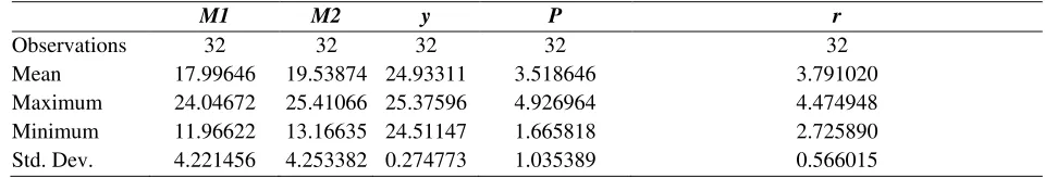
[image:4.612.67.547.469.551.2]All the data used ın this paper are delivered from the Central Bank of the Republic of Turkey (CBRT). Some basic descriptive statistics of the variables we employed in the model are presented in table 1 in logarithmic form, and general trends of variables in the model is shown in figure 1. Table 1 indicates that maximum volatility happens in narrow and broad money demand variables, and that the value between minimum and maximum is again valid for variable M1 equal to logarithm of real money balance.
Table 1: Descriptive Statistics of the variables in logartimic form
M1 M2 y P r
Observations 32 32 32 32 32
Mean 17.99646 19.53874 24.93311 3.518646 3.791020
Maximum 24.04672 25.41066 25.37596 4.926964 4.474948
Minimum 11.96622 13.16635 24.51147 1.665818 2.725890
Std. Dev. 4.221456 4.253382 0.274773 1.035389 0.566015
8 12 16 20 24 28
1980 1985 1990 1995 2000 2005 2010
M1 8 12 16 20 24 28
1980 1985 1990 1995 2000 2005 2010
M2 20 21 22 23 24
1980 1985 1990 1995 2000 2005 2010
Y 2.0 2.5 3.0 3.5 4.0 4.5
1980 1985 1990 1995 2000 2005 2010
[image:5.612.112.502.114.332.2]R
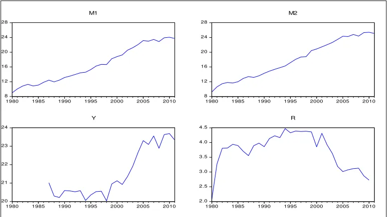
Figure 1: General trend of variables used in the model Source: Author’s drawings
3.1 Unit Root Test Result
Before estimating equation (5) we will firstly investigate stationarity and level of integration of time series we employ in the model. The determination of the degree of integration of series and the choice of appropriate cointegration analysis I (1) or I (2) is important to make appropriate econometric analysis (Güloğlu and İvrendi, 2010: 9). There are also some potential problems of using non-stationary data. Because non-stationary time series can cause spurious (non-sense) regression results, as noted by Granger and New bold (1974).For this purpose we conduct unit root tests for the logarithmic variables of model (5) by both the Augmented Dickey fuller (ADF) test and Kwiatkowski-Phillips-Schmidt- Shin (KPSS) test (Kwiatkowski et al. 1992). The test results are presented in Table 2 and 3.The ADF and KPSS test results show that all variables have unit root in their level but become stationary in their first difference, i.e. they are integrated as I (1). Also this result can be seen from the figure 1 indicating that each variable has a non-stationary trend in level.
[image:5.612.68.546.568.694.2]If two series are integrated of the same order, Johansen's (1988) procedure can then be used to test for the long run relationship between them. The procedure is based
Table 2: ADF Test Resultsa
Level First Difference
(No intercept no trend)
(Intercept) t (Intercept and
Trend)
(No intercept no trend)
(Intercept) t (Intercept and
Trend
M1 4.51 -0.51 -2.42 -1.52 -5.65* -5.54*
M2 -0.76 -2.72 -3.60** -0.61 -5.61* 0.71
y 1.00 -0.29 -2.68 -5.34* -5.76* -5.61*
r -0.00 -2.65 -1.62 -6.14* -6.00* -6.36*
a
H0: I(1) is tested against alternative hypothesis H1: I(0). The order of the first difference terms is 3.
The critical values of test statistics (, , t ) are tabulated in Fuller (1976) and MacKinnon (1996).
[image:6.612.67.547.125.247.2]*, ** and show statistically significant at 1 % and 5 %respectively.
Table 3: KPSS Unit Roots Test Resultsa
Level First Difference
(Intercept) t (Intercept and Trend) (Intercept) t (Intercept and Trend)
M1 0.74 0.21 0.11* 0.13**
M2 0.74 0.22 0.21* 0.13**
y 0.61** 0.75 0.27* 0.13*
r 0.21 0.19** 0.56* 0.8*
a
H0: I(0) is tested against alternative hypothesis H1: I(1).
Notes: Critical values are taken from Kwiatkowski-Phillips-Schmidt-Shin (1992) Table 1.
*, ** and show statistically significant at 1% and 5 % respectively.
Since all series are non-stationary, then there may beboth short- run and long-run relationships between these variables. In order to examine the existence of a short-run relationship, we should check the relevant coefficients in the Vector Autoregressive (VAR) model. But to check the existence of a long-run relationship between variables, then we will firstly perform a co-integration test.
3.2 Co-integration test result
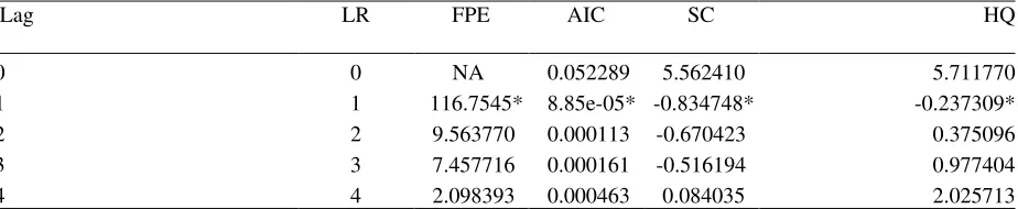
In this part we are examining whether the variables are co-integrated with each other with Johansen co-integration test. Because a linear combination of non-stationery time series could make a long run equilibrium point over time. If one or more linear combination of individually non-stationary series is stationary then these series may be co-integrated. This means that these series cannot move too far away from each other (Dickey, Jansen and Thorton, 1991:58). We firstly determine lag length of unrestricted VAR model within five different lag selection criterions including likelihood Ratio (LR), Final Prediction Error Criterion (FPE), Akaike information criterion (AIC), Schwarz information criterion (SC) and Hannan-Quinn information criterion (HQ). The maximum lag number selected is 4. Lag order selection criteria results are shown in table 4. We also add three dummies (D94, D01 and D08) as exogenous variables to the VAR model to consider the unpredicted shock effects of three economic crises occurred in 1994, 2001 and 2008 respectively. The dummy variables D94, D01 and D08 are unity for year 1994, 2001 and 2008 and zero otherwise. According to table 4, most of the lag selection criterions suggest 2 lag orders.
Table 4: Lag Selection Criteria Results
Lag LR FPE AIC SC HQ
0 0 NA 0.052289 5.562410 5.711770
1 1 116.7545* 8.85e-05* -0.834748* -0.237309*
2 2 9.563770 0.000113 -0.670423 0.375096
3 3 7.457716 0.000161 -0.516194 0.977404
4 4 2.098393 0.000463 0.084035 2.025713
* indicates lag order selected by the criterion, LR: sequential modified LR test statistic (each test at 5% level), FPE: Final prediction error, AIC: Akaike information criterion, SC: Schwarz information criterion, HQ: Hannan-Quinn information criterion,
[image:6.612.77.539.510.605.2]values of the tests are tabulated from Johansen and Juselius (1990). Table 5 presents the results of Johansen Cointegration Test using the maximum eigenvalue and the trace tests. Both the maximum eigenvalue and trace tests results shown in table 4 suggest one co-integration relationship among three variables
Table 5: Tests results for co-integration rank
H0 HA λi λmax CV 95% H0 HA Trace CV 95%
r=0 r=1 0.644078 21.69390 21.13162 r=0 r1 49.60239 29.79707 r1 r=2 0.504434 14.14317 14.26460 r1 r2 15.30849 15.49471 r2 r=3 0.465765 13.16532 3.841466 r2 r3 13.16532 3.841466
Critical values are tabulated from Table 1 of Osterwald and Lenum (1992). * shows significance level at 5%.
3.3 Estimation Results
We find that there is only one co-integrating vector between variables indicating that we can estimate long-run relationship between variables using vector error correction (VEC), DOLS and FMOLS techniques. For this purpose in this section, the long-run dynamics of money demand function of equation (5) is estimated by VEC, DOLS and FMOLS methods.
A VECM model with our variables and one lag is simply stated as follow:
( ) ( ) ( ) ( ) ( ) ( )
Where; m, r and y are at the first differenced variables, and are equal to m1 or m2. indicates constant coefficient
and and shows short run causalities, while is the long run coefficient of the VEC model. ( )is the one period lag residual of co-integrating vectors of the long run model given below:
( )
Where ( )indicates the adaptation rate to the long run equilibrium. It corrects disequilibrium and leads variables m, r and y of the system to converge its long run equilibrium point. Hence, we expect that the sign of should be negative. Because coefficient shows what rate it corrects the previous period disequilibrium of the system. Also, negative coefficient means that there is a long run relationship among variables r, y and m.
VEC estimation result of the equation (6) with one lag is reported in Table 6. The coefficient of error correction term EC (-1) is negative and significant as expected: -0.34 meaning that system corrects its previous period disequilibrium at a speed of approximately 34 percent yearly. In other saying, almost 34% of deviation from long run equilibrium is smoothed in one year. Moreover the sign of coefficient EC(-1) is significant and negative, as it is expected, indicating that there existed a long run causality from y and r to m. This result indicates that in long run income and nominal interest rate cause money demand.
Table 6: Error Correction Model Estimation Result
VEC1: Dependent variable:
m1 VEC2: Dependent variable: m2
Explanatory
variables Coefficient
Prob.
Coefficient Prob.
( ) -0.345680* 0.0000 -0.081167* 0.0097
( ) 0.599926** 0.089 1.318553* 0.0027
( ) 0.873500* 0.059 1.733377* 0.0002
( ) -0.992656* 0.0572 -1.033190* 0.0020
0.769424* 0.0000 -0.016065 0.9361 Co-integration equation:
M1(-1) = 5.65*Y(-1) - 5.159*R(-1) + 122.02
Co-integration equation:
M2(-1) = 6.46*Y(-1) -10.66*R(-1) - 159.61
According to estimation result of co-integration equations (long-run relationship) under the table 6 there is a strong and significant long run relationship between m, r and y. It implies that a percentage increase in income is associated with a 5.65 percentage increase in M1 and 6.46 percentage increase in M2. Also, a percentage increase in nominal interest rate is associated with a 5.15 percentage decrease in M1 and 10.66 percentage decrease in M2.The signs of
the short run coefficients are the same as in the long run except the constant term in VEC2 model. İt is clearly seen
that the short-run elasticities have values lower than the long run elasticities for both narrow and braod Money demand (VEC1 and VEC2 models).
Furthermore, The Stock- Watson’s DOLS model is generally used in small samples and gives a robust result compared to alternative techniques. The presence of leads and lags for different variables eliminates the bias of simultaneity within a sample and DOLS estimates and provide better approach to normal distribution (Baba et al, 2013:23). DOLS model with dependent variable yt and independent variable xt is specified as below:
∑ ( )
Where n and m show lag and lead length, and indicates the long run effect of a change in x on y. The reason why lag and lead terms are included in DOLS model is that they have the role to make its stochastic error term independent of all past innovations in stochastic repressors (Baba et al, 2013:23). Equation (5) is specified in a DOLS framework as follows:
∑ ∑
( )
Where and shows leads and lags. The optimal lag structure can be determined by using
AIC (Akaike Information Criteria), SC (Schwarz Criteria) or using the values of √ recommended by stock-Watson (1993) for DOLS approach, where N is number of observation.According to Stock-Watson’s approach the optimal lag should be equal to √ Since we have limited observation, we prefer AIC and SC criteria to determine lag length. FMOLS and DOLS estimation result is presented in table 7 suggesting that in both FMOLS and OLS models which do not include trend model, the interest rate and real national product are negatively and positively related to narrow (M1) and broad (M2) money demand as the economic theory and many other empiric studies presupposed. In both models coefficients are significant at least at 5% percent error level. Estimation result of linear models contradicts with economic theory, so we take into consideration only estimation results of the models not including linear trend.
Table7: Co-integration Estimation: DOLS and FMOLS Estimation Result Based on Econometric Model (9)
Dependent Variable: M1
Trend: None Trend: Linear
Estimation Method r y r y
DOLS -2.18** 1.24* 8.48* 6.33*
FMOLS -2.38* 1.26* 7.08* 5.70*
Dependent Variable M2
Trend: None Trend: Linear
Estimation Method r y r y
DOLS -1.71** 1.23* 10.85** 7.21**
FMOLS -1.96** 1.25* 8.60* 6.21*
Note: Leads and lags were set to 1 and 2 for DOLS estimators. **and * shows statistical significanceat 5 and 1 percent level.
Estimation results also suggest that the impact of interest rates on Money demand is greater than that that of the real product in in Turkey. We conclude that the coefficients gained from long run estimation of money demand function by Johansen co-integration method is larger than coefficients estimated by FMOLS and DOLS techniques.
4. Conclusion
The main aim of this paper is to investigate the dynamic determinants of money demand function, developed and by Bae and De Jon (2005) but based on Keynesian liquidity reference theory, for Turkey covering time period from 1980 to 2012using Johansen co-integration test, vector error correction, Dynamic Ordinary Least Squares (DOLS) and Fully Modified OLS (FMOLS) techniques.
The estimation result of the dynamic money demand function is both consistent with the earlier empirical findings and suggests that suggest that there is a long-run relationship between money demand, income and nominal interest rate as economic theory anticipates. But the long run-coefficients estimated from FMOLS and DOLS is smaller than that of the Johansen co-integration vectors. Nevertheless, real money demand in Turkey is positively related with income and negatively related with nominal interest rate. Correction procedure is very high, and corrects nearly 31 percent of the biases from long run equilibrium in one year due to shocks in the short run.
References
Adam, C. (1992). On the dynamic specification of money demand in Kenya, Journal of African Economies1, 233-270.
Asuamah S.Y, Tandoh F., Mahawiya S. (2012). Demand for Money in Ghana: An empirical assessment, Advances in Arts, Social Sciences and Education Research, Vol 2,No 7.
Baba Y, Hendry DF, Starr RM. (1992). The demand for m1 in the USA, 1960-1988. The Review of Economic Studies 59: 25–61.
Ball L. (2001). Another look at long-run money demand. Journal of Monetary Economics 47: 31–44.
Bae, Y., & De Jong, R. M. (2007). Money demand function estimation by nonlinear cointegration. Journal of Applied Econometrics, 22(4), 767-793.
Chow, G.C. (1966). On the Long-Run and Short-Run Demand for Money, Journal of Political Economy, University of Chicago Press, vol. 74.
Choi, Chi Young, Ling Hu and Masao Ogaki (2008), Robust Estimation for Structural Spurious Regressions and a Hausman-type Cointegration Test, Journal of Econometrics, Vol. pp. 142: 327-351.
Handa, J. (2009). Monetary Economics. New York: Routledge Taylor & Francis Group.
Chang Y, Park JY, Phillips PCB. (2001). Nonlinear econometric models with cointegrated and deterministically trending regressors. Econometrics Journal4(1): 1–36.
Chen SL, Wu JL. (2005). Long-run money demand revisited: Evidence from a non-linear approach. Journal of International Money and Finance 24: 19–37
Drama, B. H. G. and Yao, S. (2010). The demand for money in Cote d’Ivoire: evidence from the cointegration test, International Journal of Economics and Finance, 3(1).
Ewing, B. T. and Payne, J. E. (1999). Long-run money demand in Chile, Journal of Economic Development, 24(2), 177-190.
Eatzaz, A. and Munirs, M. (2000). An Analysis Of Money Demand In Pakistan, Pakistan Economic and Social Review, Vol. 38, No. 1, pp. 47-67.
Hoffman DL, Rasche RH. 1991. Long-run income and interest elasticities of money demand in the united states. The Review of Economics and Statistics 73(4): 665–674
Güloğlu, B. and İvrendi, M. (2010). The Effects of Monetary Policy Shocks on Exchange Rate: A Structural VECM With Long-Run Restrictions
Granger, C.W.J. and Newbold, P . (1974). Spurious Regressions in Economics, Journal of Econometrics, Vol 2/2; 111-120
Kallon, K. (1992). An econometric analysis of money demand in Ghana, Journal of Developing Areas 26, 475-488
Laidler DEW. (1985). The Demand for Money: Theories, Evidences, and Problems. Harper &Row, Publishers, New York.
Lucas Jr. RE. (1988). Money demand in the united states: A quantitative review. Carnegie-Rochester Conference Series on Public Policy 29: 1061–1079.
Mehra YP. (1993). The stability of the m2 demand function: Evidence from an error-correction model. Journal of Money, Credit, and Banking 25(3): 455–460.
Miller SM. (1991). Monetary dynamics: An application of cointegration and error-correction modeling. Journal of Money, Credit, and Banking 23(2): 139–154.
Miyao R. (1996). Does a cointegrating m2 demand relation really exist in the united states? Journal of Money, Credit, and Banking 28(3): 365–380
Nell, K. S. (2003). The stability of M3 money demand and monetary growth targets: The case of South Africa, Journal of Development Studies39, 151-180.
Park JY, Phillips, PCB. (1999), Asymptotics for nonlinear transformations of integrated time series. Econometric Theory 15(3): 269–298.
Park JY, Phillips, PCB. (2001). Nonlinear regressions with integrated time series. Econometrica 69(1): 117–161.
Pedron, P. (2000). Fully modified OLS for heterogeneous cointegrated panels, Advances in Econometrics, 15, 93– 130.i
Pedroni, P. (2001). Purchasing power parity tests in cointegrated panels, Review of Economics and Statistics, 83, 727-731.
Stock, J.H. and Watson, M. (1993). A Simple Estimator of Cointegration Vectors in Higher Order Integrated Systems. Econometrica, pp. 61, 783-820.
Sriram SS. (2001). A survey of recent empirical money demand studies. IMF Staff Papers 47(3): 334–365.