251
A differential evolution algorithm to solve new green VRP model by
optimizing fuel consumption considering traffic limitations for
collection of expired products
Mojgan Karami
1and Vahid Reza Ghezavati
1*1School of Industrial Engineering, Islamic Azad University, South Tehran Branch, Tehran, Iran
[email protected], [email protected]
Abstract
The purpose of this research is to present a new mathematical modeling for a vehicle routing problem considering concurrently the criteria such as distance, weight, traffic considerations, time window limitation, and heterogeneous vehicles in the reverse logistics network for collection of expired products. In addition, we aim to present an efficient solution approach according to differential evolution (DE) procedure to solve such a complicated problem. By using mathematical modeling tools for formulating the environmental sensitivities in vehicle routing problems, the reverse logistics must be managed according to criteria such as cargo weight carried by the vehicle, the vehicle speed and the covered distance by the vehicle. This leads to optimization and reduction of transportation fuel consumption and hence reduction of air pollution and environment concerns. This concept has led to creation and study of the green vehicle routing problems in this paper. Numerical analysis indicates that performance of the proposed DE algorithm can be validated in terms of CPU run time and optimality gap for solving the proposed model. Furthermore, sensitivity analysis show that extending maximum travelling distance by each vehicle, and increasing capacity of vehicles lead to reduction of total cost in the problem. Keywords: Green vehicle routing problem, reverse logistics, expired products, transportation system, differential evolutionary algorithm
1-Introduction
Transportation is one of the greatest parts of supplies which has irreplaceable and unchangeable fundamental infrastructure for the economic growth of a country. Overuse of energy and hence the air pollution in recent years is a warning and a threat to the environment. This has attracted the attention of transportation system players and has forced them to think about appropriate and applicable solutions in order to reduce and optimize fuel consumption of the transportation system. Achievement to these solutions helps in protection of environmental health and cost saving in the fleet fuel.
Transportation has irreparable effects on the environment. Emission of greenhouse gases and carbon dioxide from vehicles fuel directly affects the people health and can cause destruction of the ozone layer.
Journal of Industrial and Systems Engineering
Vol. 11, No.2, pp. 251- 269 Spring (April) 2018
*Corresponding author
252
Greenhouse gases from the transportation system are significant portions of air pollution in different countries of the world. Therefore, increase of concerns about these dangerous effects, shows implementation necessity of a program in the transportation system; routing models of the green vehicles based on reduction of fuel consumption and hence decrease of air pollution can be a suitable solution. Green vehicles routing problem is introduced by compatible subjects with the environment and economic costs considering the effective paths for encountering and achieving the financial indicators and environmental importance. Green vehicle routing is classified into three main groups including: green vehicle routing problem, pollution routing problem and vehicle routing problem in reverse logistics. In the rest of this paper, section 2 indicates literature survey and literature gap for motivating in this paper. Section 3 introduces mathematical formulation. The solution procedure is presented in section 4. Section 5 shows the numerical experiments and the results. Finally, section 6 summarizes the paper.
2- Literature review
During recent years, different models are proposed considering various standards for the sake of this purpose. According to the literature, vehicle speed, weight of collected expired products and the transportation distance are effective factors on the fuel consumption of transportation. Kara et al. (2007) studied the transportation real cost which is affected by the vehicle load and the covered distance. They considered the vehicle routing problem with the aim of energy reduction as a routing problem with capacity limitation and with a new purpose of cost. The cost function is product of the whole load (including curb vehicle) and the path length. They used this to facilitate the relationship between the minimum consumed energy and the variable problem situations. Xiao et al. (2012) calculated fuel cost for the transportation parts and its whole based on crude oil. They came to the conclusion that decrease of the fuel consumption and improvement of the transportation performance in a practical level are possible and presented a fuel consumption formula. They suggested the fuel consumption rate regarding the vehicle routing problem with capacity limitation and developed the vehicle routing problem with capacity limitation with the aim of fuel consumption minimization. In their suggested model, the covered paths and the load are considered as the factors which determine the fuel costs. Fuel consumption rate is considered as a function dependent to the capacity and the proposed model of fuel consumption rate is linearly continuous with the vehicle capacity. Kuo (2010) presented a time dependent model for calculation of the fuel consumption in the vehicle routing problem. In this model, three factors of transportation distance, transportation speed and the collected expired products weight have been considered. In this study, impassable paths are not overlooked while they are usually neglected in vehicle routing problems. The proposed method proposed a better path with less fuel consumption but with longer transportation times and distances. It is expressed that there may be an interaction between the fuel consumption, the transportation times and the transportation distance. Erdogan et al. (2012) considered for first time the vehicle recharge and refueling possibility in the vehicle routing problem. They showed this problem as the green vehicle routing problem in which the fuel station of the vehicle which is allowed to refueling during travel can increase the travel length. This model limits the refueling danger with the aim of minimizing the trip. They considered the service time of each customer and the maximum time limitation in each selected path. Schneider et al. (2014) studied the green vehicle routing problem with fuel consumption optimization target considering the time window. Tavares et al. (2009) investigated road slope effect and the vehicle load on the fuel consumption amount in waste collection problem and only for three levels. Half load during waste collection, complete load during going to the unloading place and without load in the return path. Relationship between the fuel consumption rate and the full load is not considered in their study. However, it is obvious that when the vehicle services to a node, its load amount reduces which results in reduction of fuel consumption rate in the path length. Therefore, considering the fuel rate dependent to the load is essential in costs accurate calculation. Suzuki (2011), in addition of considering load amount effect on the vehicle fuel consumption, investigated vehicle waiting time effect in the service beginning to costumers on the fuel consumption. Pronello et al. (2007) considered more realistic models than the previous researches in this filed for measurement of the generated pollution from the vehicle during paths that computation of more factors such as trip time when
253
the vehicle engine is cold is needed. Sbihi et al. (2007) studied a time dependent vehicle routing problem. Based on when vehicles are in the suitable speed, less pollution is provided; their control far from congestion has more compatibility with the environment; even if this leads to increase of the trip length. Palmer (2007) presented a model of carbon dioxide emission and an integrated routing and also calculated the amount of released CO2 in trip and the trip time and distance. This paper investigates dependency of speed effects in reduction of CO2 emission in different traffic scenarios with time window. Results show that about 5 percent reduction of CO2 can be achieved. Buhrkal al. (2012) performed a case study in Denmark for city garbage collecting through vehicle routing problem with time window limitation. The aim of this study was finding a path with optimized cost for city garbage collecting vehicles and garbage transmission to the waste recycling centers in a time window which meets the citizens sat is faction. Le Blanc et al. (2006) also investigated a case study about components recycling of old vehicles to optimize logistics network for collecting containers which are used in Netherland to deliver expired materials from scrappers They considered a vehicle routing model by putting several warehouses and simultaneous removal and delivery. Krikke et al. (2008) studied stock routing problem in components collection from vehicles scraps which their lifetime is ended. Use of available stock data and also stock levels are seen in this model and MUST and CAN instructions are used for creation and planning of components collecting plans. Kim et al. (2009) investigated reverse logistics flow for recycling electronic commodities that their lifetime is ended in South Korea. Demir et al. (2012) presented a great adaptive neighborhood search for pollution routing problem based on increase of consumption efficiency for vehicle routing problem with great and average sizes. Faulin et al. studied (2011) a vehicle routing problem with capacity limitation with environmental standards and considering environmental complex effects. Expect traditional economic costs measurement and environmental costs which are created by the emissions, environmental costs resulted from noise and crowd have been considered in the infrastructure.
One of the most important studies on the application of innovative methods in VRP with time windows is done by Niu et. al. (2018). They have examined different innovative approaches on this problem and compared the results. VRP with stochastic elements has received some attentions. Pierre and Zakaria (2016), Hafezalkotob et. al., (2017) and Zhang et. al. (2016) have employed stochastic optimization techniques to solve small size problems.
Some researchers integrated multi criterion decision-making techniques with routing problems. Torfi et. al. (2016) applied a new analytical technique for determining the relative weights of evaluation criteria using trapezium fuzzy numbers in, and then, the previous results integrated with a location routing problem. Gribkovskaia et al. (2008) studied a similar problem to Prive et al. (2006) with difference that each costumer has two visit permits. Aras et al. (2012) considered a multi-warehouse vehicles routing problem with removal selection and pricing during which the client selection was optional and was dependent to if the visit is profitable and if the remaining space of vehicle meets all the recycling products of the customer. Bipartite collection was illegal. Maden et al. (2010) considered vehicle routing problem with time window limitation in which the speed was dependent to the trip time. In addition, an innovative algorithm was proposed for problem solving. In their results, they achieved to 7 percent of saving in the generated carbon dioxide in a case study in England. Jabali et al. (2009) considered a problem similar to Maden with difference that the generated pollution amount is estimated based on a linear function of vehicle speed and presented an analysis to find the optimized speed considering the pollutions amount. Moreover, a prohibited repetitive search algorithm was used for solving vehicle routing problem samples. Ahmadizar et. al. (2015) proposed a model that studies two-level vehicle routing together with cross-docking. They considered transportation costs and the fact that a specified product type may be supplied by different suppliers at different prices. Bauer et al. (2010) explicitly worked on greenhouse gases minimizing greenhouse gases emissions in a multi-aspect transportation model and showed the ability of this model to reduce the greenhouse gases emissions. Fagerholt et al. (2010) attempted to demonstrate decrease of fuel consumption and carbon dioxide emission show with speed optimization in sending and transportation scenario. Considering constant transportation paths and time windows, speed of every section of the path was optimized for fuel saving. Bektas and Laporte (2011) presented a pollution problem with and without time window and a comprehensive cost function which combined minimizing
254
carbon dioxide emissions costs with drivers operating costs and fuel consumption was proposed. However, their model assumed a minimum flow speed of 40 km/h which is in conflict with the real world condition in which crowd occurs. Dell’Amico et al. (2006) defined a linear zero/one programming model and investigated the category technique and price in this problem solving. Alshamrani et al. (2007) studied a real problem of blood distribution and blood vessels collecting. Penalty cost was considered whenever these blood vessels were not picked. In addition, potential demands and periodic visits were considered in this developed model. Mingyong et al. (2010) presented a mixed planning model for vehicle routing problem with time window for commodities distribution and collection with the aim of cost saves and environment protection and solved the model with the differential evolution algorithm.
Based on the literature gap that is detected in this paper, no researches considers concurrently green considerations with some real limitations such as traffic network and time windows in order to formulate a model in the reverse logistics for collection of expired products. To fill this gap, we aim to develop a novel mathematical model in order to reduce fleet fuel consumption that has an important role in reducing air pollution. This model considers the criteria such as distance, weight, traffic network, time window limitation and heterogeneous vehicles. Finally, to solve such a complicated model an efficient meta-heuristic method based on the differential evolution algorithm will be proposed.
3-Mathematical modeling
In this section, mixed integer nonlinear programming model is presented for reduction of fleet fuel consumption which is heterogeneous and perform reverse logistics of the city expired products. Generally, to achieve this target, the criteria such as the covered distance by the vehicle, the carried load by the vehicle, traffic and vehicle speed must be considered. The following assumptions are considered:
Each customer is visited exactly once during the path
Each vehicle starts from the warehouse and gets back to there at the end of service
Total demand of each route must not overpass the vehicle capacity
Heterogeneous vehicles are considered
Number of vehicles from each type must be considered limited
The place of collecting center is fixed and is pre-defined
Vehicle speed is constant
All expired products from the customers must be collected by the heterogeneous fleet In the following, the indexes, parameters, and model decision variables are introduced.
Indexes:
n : clients node index which i,j∈n and i=0 shows depot.
v: vehicle index (v=1, 2,…, v).
r: all accessible routes index
e: work shift index (e= 1, 2, 3)
Parameters:
Qv: capacity for vehicle v,
Si: service time for customer i.
ai: earliest arrival time to the node ith.
bi: latest arrival time to the node ith.
Tijrev : trip time between nodes i,j from route r by vehicle v in the work shift e.
M: an upper bound for each constraint or decision variable.
255
Lmaxv : maximum mileage distance by vehicle vth.
pj : returned products amount from node j.
Fcijrev : unit of fuel consumption by v vehicle through r route between nodes i , j in work shift e.
𝐿1𝑒 : eth work shift beginning time for transportation.
𝐿2𝑒 : eth work shift end time for transportation.
Decision variables:
xijrev : 1 , if vehicle V travels from customer i to customer j through route r and in work shift e, otherwise 0.
yiv : all picked up demand by vehicle V in i node.
Waiev : waiting time for vehicle V in work shift e in node i.
wiev : beginning service time for vehicle V at customer i in work shift e.
iev
: 1, if Vehicle V in work shift e visit node i, otherwise 0.Then VRP model can be formulated into the mixed integer nonlinear programming model.
1
MinTF
2
s.t
1
i r e v ijrev
x
j
3
1
j r e v ijrev
x
i
4
0
i r e
jirev ijrev
x
x
j,v
5
Maxv
ij i j r e
ijrevd L
x
v
6
1
0
r j e jrev
x
v
7
0 0
0
j r e
rev j jrev x
x
v
8
0
0
j jv
y
v
9
i r e irev i j r e
ijrev M x
x 0
v
10
r e ijrev j
iv
jv
y
p
M
x
y
1
ijv
11
k
iv
Q
y
v
12
ijrev
jev iv ijrev i
iev s t wa w M x
w 1 ijrev
13
i jireve
iev
a
x
256
14
j r e jirev i
e
iev b x
w iv
15
j r ijrev e
iev L x
w 1
iev(16)
j r jirev e
iev L x
w 2
iev(17)
iev
j r e
iev ijrev
i iev
e w s x wa M
L
2
iev
(18)
j r jkrev
iev M x
wa iev
(19) iev
j r
ijrev M
x
iev(20)
e
x
e
x
k r e jkrev r e
ijrev
ijv(21) 00rev
0
r e
x
v(22)
iv
ijrev i j r e v
ijrev fc y
x
TF
1(23)
0,1 ,, v iev ijrev Se
x
(24)
0
,
,
iev iv
iev
w
y
wa
Constraint (1) which is the objective function reduces the fuel consumption of the whole fleet. Constraint (2) ensures that every demand node is entered once. Constraint (3) ensures that each demand node is departed once. Constraint (4) ensures the balance between arrival and departures of vehicle from the demand node. Constraint (5) ensures the maximum allowed distance for vth vehicle. Constraint (6) ensures that each vehicle does not exit more than once from the warehouse. Constraint (7) is ensures the balance between arrivals and departures of vehicle from the warehouse. Constraint (8) ensures that the vehicle is empty when leaving the warehouse. Constraint (9) explains that can’t go to any demand node until it leaves the warehouse. Constraint (10) shows the amount of returned product from each demand node. Constraint (11) ensures that the returned products by every vehicle should not be over its load. Constraint (12) meets service beginning limitation and fulfills demand of the next node, and also this constraint prevents cycling in the route. Constraint (13) ensures that the service beginning time occurs in the time window lower bound of the corresponding node. Constraint (14) ensures that the service beginning time is smaller than the time window upper bound of the corresponding node. In fact, constraints (13) and (14) state that service to each node must be done in the considered interval time. Constraints (15) and (16) are related to the time window of the whole service in the considered work shift interval time and represents that service must be done in the considered work shift interval time. Constraint (17) ensures that the service to the demand nodes must be done the determined work shift interval time. Constraint (18) is the logic limitation and states that there will be waiting time in a node only in case of visiting that node. Constraint (19) ensures that only when a node has a demand in an interval time, the vehicle is sent for servicing from the considered path to the considered node. Constraint (20) is the logic constraint and shows order of nodes visits and explains that the visit time of the previous
257
node is smaller than next nodes. Constraint (21) prevents occurrence of prohibited route. Constraint (22) shows fuel consumption of the transportation fleet. Constraints (23) and (24) explain variables domains.
4- Solution method
VRP problem is classified as Np-hard problems in combinatorial optimization problems (Miranda and Conceição, 2016). Differential evolution (DE) algorithm is considered as a powerful and fast method for optimization problems in continues space. It is one of newest search methods which were presented by Stone and Pries in 1995. They indicated that this algorithm has proper ability in optimization of differentiable nonlinear functions. This algorithm is presented to cover the main defect of genetic algorithm which is lack of local search. In the selection operator of genetic algorithm, chance of response selection, as one of the parents, depends on competency. It means that their selecting chance depends on their competency. When a new response is generated by using a self-regulation mutation and intersection operator, the new response will be compared to the previous one and will be replaced in case of being better. One of the benefits of this algorithm is having a memory which keeps suitable solutions data in recent population. Other advantage of this algorithm is related to the operation selection. In this algorithm, all responses have a same chance to be chosen as one of the parents. The algorithm stages are as following:
4-1- Initiation population
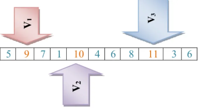
One of most important components in the recommended solution algorithm is the representation structure of the problem responses. Since the problem responses must indicate service routes to sets of customers, hence if the clients' number in n and the vehicles’ number in v, then the response representation is the permutation solution of n customers with (v-1) vehicles which has used rand perm function. In continuation, by using the FIND function which a value greater than n, the response will obtained and interpreted as follows:
N=8 and V=4 is a permutation as in following and are interpreted as follows:
Fig 1. Permutation for N=8 and V=4
In the solution representation, total number of nodes is n + (v-1) where n denotes number of customers and v indicates number of vehicles. In the shown permutation, numbers 1, 2, …, 8 denotes number of customers nodes and numbers 9, 10 and 11 denotes number of vehicles nodes.
Customers 6 and 3 are covered by vehicle 3 that is located in node 11; customers 4, 6 and 8 are covered by vehicle 2 that is located in node 10. Customers 1 and 7 are covered by vehicle 1 that is located in node 9. Customer 5 is covered by vehicle 4 that is located in node 12 where node is not shown. The constraints 2, 3, 4, 6, 7, 21 are regarded with this chromosome. In continuation of the program, this chromosome is reviewed in 20,…, 9, 5 constraints. A penalty function is considered if the constraints are not met. Therefore, in case of customer visit before the time window beginning, the vehicle must decide to service out of the time window and take the second demand or wait until the time window beginning. If this limitation is not met, its penalty function is zero. Otherwise, it will be fined according to the prolongation
6
3
11
8
6
4
10
1
7
9
5
V3
2
V
258
time and exit of the considered time-window. It should be mentioned that selection of the work shift numbers is asked from the customer and a choice will be considered for vehicle and path selection which has the least fuel consumption.
4-2- Fitness function
To use the concept of a response dominancy over another response and also to rank the responses, it is needed to calculate the total fuel consumption which used by a vehicle in different tours for every response. This amount which is particular for every response is sum of the tours’ total fuel consumption and the displaced load. As mentioned, in this paper, the penalty strategy is used to prevent infeasible solutions occurrence. Sum of penalty costs is added to the objective values. Used penalty parameters are fault penalty for each capacity unit of the vehicle and also fault per every violation unit from the maximum trip time for each vehicle and the allowed travel for every vehicle.
4-3- Mutation operation
The aim of this operator is search of more points in the solution space and prevention from early convergence. After generation of the initial solutions, in this step, considering DE algorithm structure, 3 chromosomes must be chosen randomly from the population and the new chromosome is as follows:
vChrom(a,:)beta×[Chrom(b,:)Chrom(c,:)]
It should be noted that the considered chromosome is of the sequential kind. Therefore, with this formula, the values like [-71, 13, 2, 3.36, 3, 5.55, 14, 8.23, 3, 4.678, 10]may be obtained which are not acceptable and are rejected according to the integer order criterion(IOR) rule; thus, an operations is done for correcting, making positive and preventing from over passing the value of n+v-1, the number of considered nodes. Finally, application of this operator needs regulation of the mutation rate parameter, beta. In this paper, this value is considers 0.5.
Example:
2
3
1
8
6
4
10
7
9
5
5
4
2
3
1
8
6
10
9
7
3
5
9
8
6
4
10
1
2
4
4
2
6
-3
1
8
6
16
16
8
According to the obtained node negative values, duplicate and larger amounts resulting from the number of nodes that are unacceptable، By law IOR This chromosome to a chromosome becomes acceptable and The chromosomes for crossover operator used.
2
1
-7
-5
-5
-4
4
-9
7
3
10
9
7
5
4
2
3
1
6
8
a b
c
b-c
a+(b-c)
259
4-4- Crossover operation
After the mutation operation of DE algorithm, interaction operation must be done according to the following equation. The interaction rate is considered as 0.2 pcr.
Chrome(jG+1) = {chrom(j
G+1) rand(j) ≤ per
chrom(jG+1) otherwise
RAND (i) is a random value between 1 and n+v-1. In this way, using the new generation of interaction operator, the selection is placed in the evaluation function and will be in the set of optimized solutions in case of being better.
4-5- Algorithm stop condition
Finally, the number of algorithm execution must be regarded. In this paper, the strategy of implementation number is considered which evaluates 100 times by considering 50 people as the primary population.
5- Model numerical experiments
In this section, validation of the model and the proposed solution method is considered. To do so, the developed solution method in large, average and small sizes is compared with the obtained exact solution from the Gams software. Then, the model sensitivity will be analyzed.
5-1- Evaluation of the solution method in small and large sizes
In this section, performance of the proposed algorithm will be investigated. In order to do so, two problem groups are designed: one in the small size and one in the large size. In the first group, a group of sample problems are solved by the proposed meta-heuristic algorithm and results are compared with the model solution results of Gams software. The first examination target is investigating the ability of the proposed method in obtaining the optimized responses. In the second group, performance of the proposed meta-heuristic algorithm is studied in large problems with real sizes. Also, programs execution is done by a computer with CPU of 2.5 GHz and internal memory of 4.5 GB. Related value of the earliest arrival time to the customer is 0. Latest arrival time to the customer is calculated randomly by the uniform distribution of parameters 10 and 12. Amount of expired products which are collected from each customer is calculated randomly by using the uniform distribution in interval of 10 and 40. Customer service time is obtained randomly by using the uniform distribution of 1 and 4. Trip time between two nodes is calculated randomly by the multiplication of vehicle kind, route, work shift and distance between two customers, fuel consumption amount is obtained randomly by the multiplication of vehicle kind, rout, work shift, distance between two customers and the uniform function between 0.8 and 1.2. Customers servicing is done in three working shifts during a day and night. Vehicle capacity is specified according to the vehicle kind and that the maximum distance that each vehicle can travel is 100; and 1000 is a considered as a large number.
22 samples are solved by the Gams software and the differential evolution (DE) algorithm in small and medium sizes are compared in the Table (1). In this table, the first column represents the problem number; the second and the third columns are the costumer index and the route index, respectively; the fifth and sixth ones show the vehicle index and the value of the objective function which is obtained from running each specimen; the seventh column is the running time of each specimen by the Gams software which is considered as 1800 seconds in this study. Column 8 is the value of the objective function which is resulted from running the specimen by the proposed differential evolution algorithm and the next column shows the time needed for running the algorithm. Column 10 calculates the gap between DE algorithm and the Gams. In other words, this measurement indicates the percent of achieving the optimal solution by the proposed DE algorithm. Column 11 presents the run time of DE algorithm against run time of the Gams Software. Finally, the last column shows the error message of running Gams.
260
The procedure of generating all parameters is described by the following rules.
No. of customers Random uniform integer number from interval (4, 22) No. of vehicles Random uniform integer number from interval (2, 5) Amount of returned products amount from node j random uniform integer number from interval (35, 160) Vehicle capacity Random selection of scenarios 20, 30, 40
the distance between nodes i,j, Random uniform integer number from interval (2, 12)
Table 1. Comparison between the GAMS performance and the proposed DE (optimality and runtime)
G A M S e rr o r mess ag e
Comparison (DE/GAMS DE-Baron) DE GAMS DE-Baron Indices P roblem
number ( )
DE GA MS (1 DE GAMS)
GAMS Runtime Objective value Runtime Objective value V eh ic le s S h if t w o rk R o u te C u st o mers Runtime Objective value - 0.313 1 10.19 6899 32.54 6899 2 1 2 4 1 - 0.2981 1 13.43 7260 45.04 7260 2 1 2 5 2 - 0.2209 1 14.77 5828 66.84 5828 3 1 2 5 3 - 0.1886 1 14.19 5487 75.21 5487 2 2 2 5 4 - 0.1277 1 13.09 5217 102.49 5217 3 2 2 5 5 - 0.1236 1 16.77 6244 135.66 6244 2 2 2 6 6 - 0.1091 1 18.36 8592 168.19 8592 3 2 2 6 7 - 0.1005 0.967541 23.32 10942 232.04 10598 3 2 2 7 8 - 0.1006 0.978697 24.73 10474 245.69 10256 3 2 3 7 9 - 0.10731 0.962967 37.39 10221 348.43 9856 3 2 3 7 10 - 0.1156 0.953218 48.72 10850 421.36 10365 3 2 3 10 11 - 0.1235 0.912517 66.91 11076 541.66 10185 4 3 3 12 12 - 0.1004 0.946247 70.14 13994 698.42 13268 4 3 3 13 13 - 0.0992 0.933736 76.34 15721 769.04 14744 4 3 3 15 14 - 0.0808 0.943648 79.36 19708 981.28 18657 4 3 4 16 15 - 0.0709 0.927722 81.84 22001 1154.18 20518 4 3 4 17 16 - 0.0522 0.913647 86.14 22738 1648.65 20931 4 3 4 19 17 - 0.0512 0.893657 88.64 23238 1730.96 21005 4 3 4 20 18 - 0.0526 0.888162 92.99 24983 1765.33 22470 5 3 4 20 19 - 0.0570 0.902546 96.36 28438 1690.11 25913 4 3 4 21 20 - 0.0573 0.912598 102.35 29508 1785.25 27136 5 3 4 21 21 Resource limit exceeded 0.0612 0.955907 110.28 29812 1800 28553 5 3 5 22 22 - 0.0526 0.8881 - - - - - - - - Min - 0.1187 0.9542 - - - - - - - - Mean - 0.313 1 - - - - - - - - Max
261
From table 1, it is found that the proposed DE algorithm is able to reach to optimal solution by 95.42% (in average) accuracy for small and medium examples. In addition, ratio of run time for DE algorithm against Gams solver is 0.1187 that indicates DE algorithm is faster that Gams solver to find the best solution.
Fig 2. DE vs. GAMS
Considering figure 1, the exact time solution increases exponentially while the size of problems increases. Comparing the exact solution time and the time of Meta-heuristic algorithm from figure (1) and table (1), it can be seen that Meta-heuristic algorithm has reached to 95% of optimal solution after only 12% of exact time solution. This result makes the applicability of the algorithm clear.
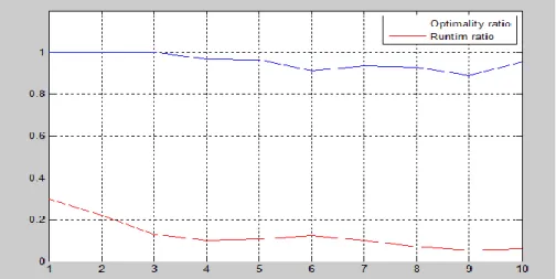
Fig 2. Descending trend of the relative optimality and runtime ratios
The above figure shows the optimization processes and the solution time. From this figure, it can be said that the slope decrease versus time is greater than the optimization process decrease. This leads to the conclusion that the meta-heuristic algorithm is very applicable.
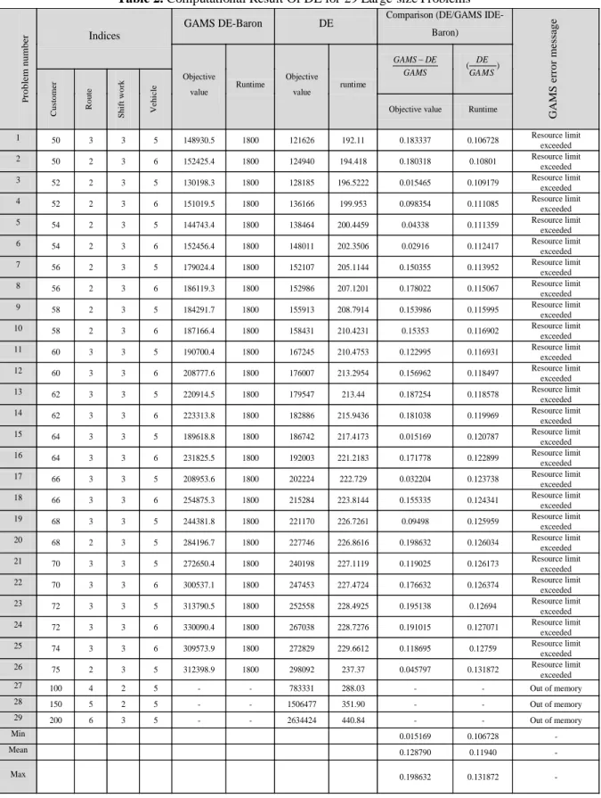
29 samples of large problems have been solved by Gams and the proposed differential evolution algorithm and the results were shown in table (2). It can be found that the Gams software reports the best solution (not optimal solution) of 26 problems during 1800 seconds that time limitation is considered for running the software, while differential evolution algorithm solved all the problems in a small amount of time. From table 2, solutions found by the proposed DE algorithm are 12.88% better than best solutions found by Gams software during 1800 seconds time limitations. Furthermore, once size of an examples
262
increases more (examples 27, 28 and 29), Gams software cannot find the best solution while DE algorithm can do it.
Table 2. Computational Result Of DE for 29 Large-size Problems
GA M S e rro r m e ss a g e
Comparison (DE/GAMS IDE-Baron) DE GAMS DE-Baron Indices P ro b le m n u mb e r
( DE ) GAMS GAMS DE GAMS runtime Objective value Runtime Objective value Ve hicle S hif t wo rk R oute C us tom e r Runtime Objective value Resource limit exceeded 0.106728 0.183337 192.11 121626 1800 148930.5 5 3 3 50 1 Resource limit exceeded 0.10801 0.180318 194.418 124940 1800 152425.4 6 3 2 50 2 Resource limit exceeded 0.109179 0.015465 196.5222 128185 1800 130198.3 5 3 2 52 3 Resource limit exceeded 0.111085 0.098354 199.953 136166 1800 151019.5 6 3 2 52 4 Resource limit exceeded 0.111359 0.04338 200.4459 138464 1800 144743.4 5 3 2 54 5 Resource limit exceeded 0.112417 0.02916 202.3506 148011 1800 152456.4 6 3 2 54 6 Resource limit exceeded 0.113952 0.150355 205.1144 152107 1800 179024.4 5 3 2 56 7 Resource limit exceeded 0.115067 0.178022 207.1201 152986 1800 186119.3 6 3 2 56 8 Resource limit exceeded 0.115995 0.153986 208.7914 155913 1800 184291.7 5 3 2 58 9 Resource limit exceeded 0.116902 0.15353 210.4231 158431 1800 187166.4 6 3 2 58 10 Resource limit exceeded 0.116931 0.122995 210.4753 167245 1800 190700.4 5 3 3 60 11 Resource limit exceeded 0.118497 0.156962 213.2954 176007 1800 208777.6 6 3 3 60 12 Resource limit exceeded 0.118578 0.187254 213.44 179547 1800 220914.5 5 3 3 62 13 Resource limit exceeded 0.119969 0.181038 215.9436 182886 1800 223313.8 6 3 3 62 14 Resource limit exceeded 0.120787 0.015169 217.4173 186742 1800 189618.8 5 3 3 64 15 Resource limit exceeded 0.122899 0.171778 221.2183 192003 1800 231825.5 6 3 3 64 16 Resource limit exceeded 0.123738 0.032204 222.729 202224 1800 208953.6 5 3 3 66 17 Resource limit exceeded 0.124341 0.155335 223.8144 215284 1800 254875.3 6 3 3 66 18 Resource limit exceeded 0.125959 0.09498 226.7261 221170 1800 244381.8 5 3 3 68 19 Resource limit exceeded 0.126034 0.198632 226.8616 227746 1800 284196.7 5 3 2 68 20 Resource limit exceeded 0.126173 0.119025 227.1119 240198 1800 272650.4 5 3 3 70 21 Resource limit exceeded 0.126374 0.176632 227.4724 247453 1800 300537.1 6 3 3 70 22 Resource limit exceeded 0.12694 0.195138 228.4925 252558 1800 313790.5 5 3 3 72 23 Resource limit exceeded 0.127071 0.191015 228.7276 267038 1800 330090.4 6 3 3 72 24 Resource limit exceeded 0.12759 0.118695 229.6612 272829 1800 309573.9 6 3 3 74 25 Resource limit exceeded 0.131872 0.045797 237.37 298092 1800 312398.9 5 3 2 75 26
Out of memory -288.03 783331 -5 2 4 100 27
Out of memory -351.90 1506477 -5 2 5 150 28
Out of memory -440.84 2634424 -5 3 6 200 29 -0.106728 0.015169 Min -0.11940 0.128790 Mean -0.131872 0.198632 Max
263
5-2- Solution of a small sample problem
Now in this second part, solution of a small size problem is described. Indexes of the customer nodes, vehicle type, working shift and route are listed in the table below.
Table 3. Sample indexes
i,j = 0,1,2,3,4,5 V = 1,2,3 r = 1,2 e = 1
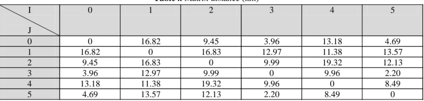
The following table displays the matrix of the distance between nodes i and j. The matrix row shows the customer i and the matrix column represents the customer j. For example, i = 0, j = 2 = 9.45 means that the distance between the customer and the warehouse is 9.45km and the remaining distances are in the same order.
Table4. Matrix distance (km)
Some parameters and variables that are mostly paid attention and affect the fuel consumption can be seen in the following tables.
Table 5. Variable values yiv (kg)
Raw of above table represents the vehicle v and its column shows customer i. For example,y1,2=50demonstratesthatthe expired products which are collected from the beginning to the second customer by the second vehicle is 50kg;and also the vehicle capacity is 100 kg.
Table 6. Variable values Wiev
W112=29 means that the beginning time of the second vehicle to the first customer service in the first working shift is second29. It should be mentioned that the day is divided into three working shifts and in this working shift, L1 = 0 and L2 = 480.
5 4
3 2
1 0
I J
4.69 13.18
3.96 9.45
16.82 0
0
13.57 11.38
12.97 16.83
0 16.82
1
12.13 19.32
9.99 0
16.83 9.45
2
2.20 9.96
0 9.99
12.97 3.96
3
8.49 0
9.96 19.32
11.38 13.18
4
0 8.49
2.20 12.13
13.57 4.69
5
2 1
𝐲𝒊𝒗
50 1
21 2
28
3
63 4
76 5
Value v
E
I
29 2
1 1 W
49 2
1 4
W
65 2
1 5
264
Table 7. Parameter values Pj (kg)
j
p J
0 0
29 1
21 2
28 3
13 4
13 5
The above table shows first column show the customer j and the second column illustrates the value pj. p1=29 means that amount of the expired products of the first customer is 29 kg.
Now, by keeping some parameters constant and changing the other parameters, the effect on the fuel consumption is investigated.
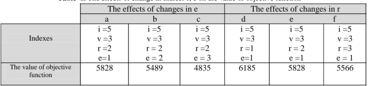
Table 8.The effects of change in indices r, e on the value of objective function
As it is obvious in the above table, by keeping the indexes i, v, r constant and changing the parameter e
which its results are brought in columns2,3and4,reduction of the objective function by changing the working shifts states that the working shift and hence the reduction of the objective function play an important role. In this manner, the results of columns4, 5 and6alsorepresentthat by keeping the indexes i,
v, e constant and route increase, fuel consumption reduction and objective function decrease are accepted.
5-3- Schematic view of the customer visit
In figure 3, the order of customer visit by vehicles is illustrated where D represents the warehouse, C1is the first customer, C2is the second customer, C3is the third customer, C4is the fourth customer and finally, the fifth customer is displayed by C5.Forbetter understanding, the figure 3(a) is being explained. In this figure, as it can be seen, the first vehicle begins its trip from the depot to the second customer through the first path; then, from the second customer to the first customer via the first path and from the first customer to the fourth customer through the first path and at the end from the fourth customer to the warehouse via the first path. In continuation, the second vehicle leaves the warehouse to collect the expired products of the two remaining customers and goes to the third customer through the first path and continues to the fifth customer from the same path and finally, it returns to the warehouse via the same path after collecting the expired products from the fifth customer.
The effects of changes in r The effects of changes in e
d e f a b c
i =5 v =3 r =3 e = 1 i =5
v =3 r = 2 e =1 i =5
v =3 r =1 e=1 i =5
v =3 r =2 e = 3 i =5
v =3 r = 2 e = 2 i =5
v =3 r =2 e=1
Indexes
5566 5828
6185 4835
5489 5828
The value of objective function
265
Fig 3.Schematic view of the customer visit
5-4- Sensitivity Analysis
In this part, step-change is performed on the model parameters which have essential role on the vehicle fuel. Parameters sin each stage has been increased to 0.2, separately. Thus, a sensitivity analysis is being done focusing on parameters LMax v and Qv and
Fc
ijrev in the Gams.Parameter
Max v
L Sensitivity Analysis of
-1 -4 -5
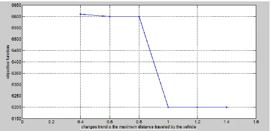
Fig 4. Changes in the objective function to change maximum distance traveled by the vehicle
As specified in the figure 4, with increasing LMaxv, feasible space becomes larger and this makes it possible to make the better solution. Therefore, it is expected that with increasing LMaxv, the objective
266
function is improved. The figure shows that with increasing LMaxv, the objective function is reduced until LMaxv equals to 1 which is its assumed value in the problem. In this case, the objective function value is reached to its minimum value and in fact, the constraints of LMaxv are relaxed.
Parameter
v
Sensitivity Analysis of Q
-2 -4 -5
In this case, it can be seen that by increasing Qv, the total amount of vehicle fuel capacity is reduced. This shows that by increasing the amount of Qv, feasible space of the problem response increases and this makes it possible to find better solutions.
Fig 5. Changes in the objective function to change vehicle capacity
arameter p
ijrev
Fc
nalysis of a
Sensitivity
-3 -4 -5
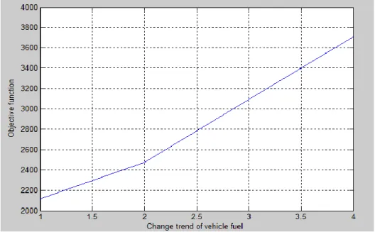
Fig 6. Changes in the objective function to change vehicle Fuel
According to the definition of FC, it is obvious that with the fuel increase for moving from node i to node j via route r by vehicle v in the working shift of e, the total fuel consumption of the fleet will
267
increase. This is evident in the figure and it can be seen that the value of objective function increases with the increase of FC.
6- Conclusion
Transportation is one of the most important parts of the supply chain which has non- replaceable substructure and is an alternative for economic growth of each country. Generally, the aim of vehicle routing problem is to affect economically the transportation routes to organize transportation services. Therefore, the use of energy and hence the air pollution are serious threats during recent years.
These threats and warnings have made the researchers to pay attention to the transportation fields seriously and think to proper and applicable solutions and to reduce the fleet fuel consumption and to optimize the transportation system. Green vehicle routing problem is related to vehicle routing problem is about the fuel consumption. Logistic activities such as expired products collecting can have great effect on the environment and therefore more friendly practical methods are used for the environment. This can lead to great achievements like environment protection and cost saving of the fleet fuel. In this paper, a model is presented for reduction of fleet fuel consumption which are heterogeneous and reverse logistics of the city expired products was planned. Generally, to achieve this target, the criteria like the covered distance by vehicle, the carried weight by vehicle, traffic, vehicle speed are considered. To represent this model, the criteria such as distance, weight, and traffic and time window are regarded. This operation is done in a level of factory and customer. The model is solved by DE algorithm and the Gams software the results were presented. The results showed that differential evolution algorithm works more efficient than the Gams software.
In this paper, reverse logistics in a single-level system showed the potential to be used in future research for the reverse logistics multi-level system.
Further research may focus on different topics including:
Periodic VRP under uncertainties in vehicles availability can be examined.
A new recovery model in case of crisis and occurrence of any scenarios can be proposed. Developing the proposed model in which scheduling resources time and employees abilities canbe considered.
References
Alshamrani, A., Mathur, K., and Ballou, R. H. (2007). Reverse logistics: simultaneous design of delivery routes and returns strategies. Computers and Operations Research, 34, 595–619.
Ahmadizar, F., Zeynivand, M., and Arkat, J. (2015), Two-level vehicle routing with cross-docking in a three-echelon supply chain: A genetic algorithm approach, Applied Mathematical Modelling, 39 (22), Pages 7065-7081.
Aras, N., Aksen, D., and Tekin, M. T. (2011). Selective multi-depot vehicle routing problem with pricing. Transportation Research Part C: Emerging Technologies, 19,866–884.
Bauer, J., Bektas_, T., and Crainic, T. G. (2010). Minimizing greenhouse gas emissions in intermodal freight transport: an application to rail service design. Journal of the Operational Research Society, 61, 530–542.
Buhrkal, K., Larsen,A.,and Ropke,S.(2012). The waste collection vehicle routing problem with time windows in a city logistics context. Procedia - Social and Behavioral Sciences 39 , 241 – 254.
Bektas_, T., and Laporte, G. (2011). The pollution-routing problem. TransportationResearch Part B, 45, 1232–1250.
268
Dell’Amico, M., Righini, G., and Salani, M. (2006). A branch-and-price approach to the vehicle routing problem with simultaneous distribution and collection. Transportation Science, 40, 235–247.
Demir, E., Bektas_, T., and Laporte, G. (2012). An adaptive large neighborhood search heuristic for the pollution-routing problem. European Journal of Operational Research, 223, 346–359.
ErdoŸan, S., and Miller-Hooks, E. (2012). A green vehicle routing problem. Transportation Research Part E: Logistics and Transportation Review, 48(1)100–114.
Fagerholt, K., Laporte, G., and Norstad, I., (2010). Reducing fuel emissions by optimizing speed on shipping routes. Journal of the Operational Research Society, 61, 523–529.
Faulin, J., Juan, A., Lera, F., and Grasman, S. (2011). Solving the capacitated vehicle routing problem with environmental criteria based on real estimations in road transportation: a case study. Procedia – Social and Behavioral Sciences, 20,323–334.
Gribkovskaia, I., Laporte, G., and Shyshou, A. (2008). The single vehicle routing problem with deliveries and selective pickups. Computers and Operations Research,35, 2908–2924.
Ashkan Hafezalkotob; Reza Mahmoudi; Mohammad Shariatmadari, (2017), Vehicle Routing Problem in Competitive Environment: Two-Person Nonzero Sum Game Approach, Journal of Industrial and Systems Engineering, 10(2). PP: 35-52
Jabali, O., Van Woensel, T. and de Kok, A.G. (2009). Analysis of travel times and CO2 emissions in time dependent vehicle routing. Tech. rep., Eindhoven University of Technology.
Krikke, H., le Blanc, I., van Krieken, M., and Fleuren, H., (2008). Low-frequency collection of materials disassembled from end-of-life vehicles: on the value of on-line monitoring in optimizing route planning.
International Journal of Production Economics, 111, 209–228.
Kim, H., Yang, J., and Lee, K., (2009). Vehicle routing in reverse logistics for recycling end-of-life consumer electronic goods in South Korea. Transportation Research Part D: Transport and Environment, 14, 291–299.
Kuo , Y., (2010). Using simulated annealing to minimize fuel consumption for the time-dependent vehicle routing problem. Computers and Industrial Engineering,59(1), 157–165.
Kara, I., Kara, B., and Yetis, M., (2007). Energy minimizing vehicle routing problem. Lecture notes in computer science (Vol. 4616, pp. 62–71).
Le Blanc, I., van Krieken , M., Krikke, H., and Fleuren, H. (2006). Vehicle routing concepts in the closed-loop container network of ARN – a case study. OR Spectrum, 28, 53–71.
Maden, W., Eglese, R., and Black, D., (2010). Vehicle routing and scheduling with time varying data: a case study. Journal of the Operational Research Society, 61,515-522.
Mingyong, L. and Erbao , C.(2010). An improved differential evolution algorithm for vehicle routing problem with simultaneous pickups and deliveries and time windows. Engineering Applications of Artificial Intelligence 23, 188–195.
Miranda, D.M., and Conceição, S.V., (2016), The vehicle routing problem with hard time windows and stochastic travel and service time, Expert Systems with Applications, 64, Pages 104-116
269
Yunyun Niu, Zehua Yang, Ping Chen, Jianhua Xiao, (2018), Optimizing the green open vehicle routing problem with time windows by minimizing comprehensive routing cost, Journal of Cleaner Production, 171, Pages 962-971
Djamalladine Mahamat Pierre, Nordin Zakaria, (2016), Stochastic partially optimized cyclic shift crossover for multi-objective genetic algorithms for the vehicle routing problem with time-windows,
Applied Soft Computing, Available online, Doi: 10.1016/j.asoc.2016.09.039
Pronello, C., and André, M. (2000). Pollutant emissions estimation in road transport models. INRETS-LTE Report, Vol. 2007.
Palmer, A. (2007). The development of an integrated routing and carbon dioxide emissions model for goods vehicles. Ph.D. Dissertation, School of Management, Cranfield University.
Privé, J., Renaud, J., Boctor, F., and Laporte, G., (2006). Solving a vehicle-routing problem arising in soft-drink distribution. Journal of the Operational Research Society, 57, 1045–1052.
Suzuki, Y. (2011). A new truck-routing approach for reducing fuel consumption and pollutants emission,
Transportation Research Part D, 16, 73–77.
Schneider, M., Stenger, A., and Goeke D., (2012). The electric vehicle routing problem with time windows and recharging stations. Technical Report, University of Kaiserslautern, Kaiserslautern, Germany.
Sbihi, A., and Eglese, R. W., (2007). Combinatorial optimization and green logistics.4OR: A Quarterly Journal of Operations Research, 5, 99–116.
Schultmann, F., Zumkeller, M., and Rentz, O. (2006). Modeling reverse logistic tasks within closed-loop supply chains: an example from the automotive industry. European Journal of Operational Research, 171, 1033–1050.
Taveares, G., Zaigraiova, Z., Semiao, V., and da Graca Carvalho, M. (2008). A case study of fuel savings through optimization of MSW transportation routes. Management of Environmental Quality: An International Journal, 19, 444–454.
Torfi, F., Zanjirani Farahani, R., and Mahdavi,. I., (2016), Fuzzy MCDM for weight of object’s phrase in location routing problem, Applied Mathematical Modelling, 40 (1), Pages 526-541.
Ubeda, S., Arcelus, F. J., and Faulin, J. (2011). Green logistics at Eroski: A case study. International
Journal of Production Economics, 131, 44–51.
Xiao, Y., Zhao, Q., Kaku, I., and Xu, Y. (2012). Development of a fuel consumption optimization model for the capacitated vehicle routing problem. Computers and Operations Research, 39(7), 1419–1431.
Junlong Zhang, William H.K. Lam, Bi Yu Chen, (2016), On-time delivery probabilistic models for the vehicle routing problem with stochastic demands and time windows, European Journal of Operational Research, 249(1), Pages 144-154