Reference group genetic algorithm for flexible job shop scheduling problem with multiple objective functions

153

Reference group genetic algorithm for flexible job shop

scheduling problem with multiple objective functions

* 1

Beheshtinia

, Mohammad Ali

1

Niloofar Ghazivakili

Industrial Engineering Department, Semnan University, Semnan, Iran 1

[email protected], [email protected]

Abstract

This article studies flexible job-shop scheduling problem (FJSSP) considering three objective functions. The objectives are minimizing maximum completion time (Cmax), the maximum machine workload (Wmax), and the total workload (WT). After presenting the mathematical model of the problem, a genetic algorithm called Reference Group Genetic Algorithm(RGGA) is used to solve the problem. RGGA implements the reference group concept in the sociology to the genetic algorithm. The term of “reference group" is credited to sociologist Robert K. Merton. Three standard data sets are used to evaluate the performance of RGGA. On the first data set, RGGA is compared to six algorithms in the literature, on the second data set RGGA is compared to four algorithms in the literature, and on the third data set RGGA is compared to three algorithms in the literature. Moreover, RGGA is compared with optimum solution in small size problem. Results show the superiority of RGGA in comparison to other algorithms.

Keywords:

1-Introduction

As industries are facing increasingly competitive situations, many classical manufacturing systems shift to newer environments such as flexible job-shop scheduling problem (FJSSP). Flexible job-shop scheduling problem is similar to the classical job-shop scheduling problem (JSSP), but FJSSP is more complex than JSSP because for each operation, it should select a machine from a set of candidate machines. This is known as the main difference between JSSP and FJSSP. FJSSP generally appears in the actual manufacturing environment. In recent years, many researchers have applied meta-heuristic algorithms to solve FJSSP.

This article considers a flexible job-shop scheduling problem (FJSSP) with three objectives and proposes a genetic algorithm called Reference Group Genetic Algorithm (RGGA) which implements the reference group concept in the sociology on the genetic algorithm. This concept indicates that people in the society imitate some reference group named “role model”. A role model is a person whose behaviors, acts or successes are or can be emulated by others, especially by youngsters. This concept is introduced by sociologist Merton (2011). Merton hypothesized that individuals compare themselves with some reference groups of people called “role models” who occupy the social role to which the individual aspires (Najian and Beheshtinia, 2018).

An example being the way fans (often times youth) will idolize and imitate professional athletes or celebrities.

*Corresponding author

ISSN: 1735-8272, Copyright c 2018 JISE. All rights reserved Journal of Industrial and Systems Engineering

Vol. 11, No. 4, pp. 153-169 Autumn (November) 2018

154

Firstly, Beheshtinia et al. (2018) implement Merton’s theory on RGGA to solve supply chain scheduling problem and dome research adapt it for other problems (Najian and Beheshtinia, 2018, Farazmand and Beheshtinia, 2018). In this research RGGA is adapted to solve flexible job-shop scheduling problem.

The rest of this paper is organized as follows: literature review (Section 2), research methodology (Section 3), results algorithm (Section 4), discussion and conclusion (Section 5).

2- Literature review

Many studies in the field of FJSSP have been presented in recent years. Shi-Jin et al. (2008) developed a filtered-beam-search-based heuristic algorithm (named as HFBS) to find sub-optimal schedules within a reasonable computational time for the FJSSP with multiple objectives of minimizing makespan, the total workload of machines and the workload of the most loaded machine. Ong et al. (2005) consider an artificial immune algorithm (AIA), named ClonaFLEX, using the clonal selection principle to solve FJSSP. Kacem et al. (2002) proposed a localization approach to solve the resource assignment problem, and an evolutionary approach controlled by the assignment model to solve FJSSP. Xia and Wu (2005) suggested a hybrid approach to solve multi objective FJSSP. The approach uses a particle swarm optimization (PSO) algorithm to assign operations to machines and a simulated annealing (SA) algorithm to schedule operations on each machine.

Gen et al. (2009) proposed a multistage operation algorithm based on GA. Bożejko et al. (2010) dealt with the FJSSP by using a parallel TS based meta-heuristics algorithm which treats routing and sequencing separately.

Bagheri et al. (2010) presented an integrated approach based on artificial immune algorithm (AIA). This algorithm uses several strategies for generating the initial population and selecting the individuals for reproduction. Also, different mutation operators are used to reproduce new individuals. To show the effectiveness of the proposed method, numerical experiments using benchmark problems are used. Pezzella et al. (2008) developed a genetic algorithm to solve FJSSP, in which a mix of different rules is used to generate the initial population, selection of individuals, and reproduction operators.

De Giovanni and Pezzella (2010) proposed an improved genetic algorithm to solve the distributed and flexible job-shop scheduling problem.

Al-Hinai and ElMekkawy (2011) addressed the problem of finding robust and stable solutions for the flexible job shop scheduling problem with random machine breakdowns and propose two-stage Hybrid Genetic Algorithm (HGA) to generate schedule. Moslehi and Mahnam (2011) presented a new approach based on a hybridization of the particle swarm and local search algorithm to solve the multi-objective flexible job-shop scheduling problem.

Combining the chaos particle swarm optimization with genetic algorithm, Tang et al. (2011) proposed a hybrid algorithm. Chen et al. (2012) developed a scheduling algorithm for job shop scheduling problem with parallel machines and reentrant process. A real weapons production factory is used as a case study to evaluate the performance of the proposed algorithm. Karimi et al. (2012) proposed a knowledge-based meta-heuristic algorithm, called knowledge-based variable neighborhood search (KBVNS) to solve FJSSP. Wang et al. (2012) applied the artificial bee colony (ABC) algorithm and estimation of distribution algorithm (EDA) to the FJSSP, both of which stress the balance between global exploration and local exploration. Zhang et al. (2012) proposed a model for Flexible Job Shop Scheduling Problem (FJSSP) with transportation constraints and bounded processing times. A genetic algorithm with tabu search procedure is proposed to solve both assignment of resources and sequencing problems on each resource. Chiang and Lin (2013) addressed the multi objective flexible job shop scheduling problem (MOFJSSP) regarding minimizing the makespan, total workload, and maximum workload. Huang et al. (2013) considered the due window and the sequential dependent setup time.

Li and Pan (2013) proposed a hybrid chemical-reaction optimization (HCRO) algorithm for solving the job-shop scheduling problem with fuzzy processing time. In the proposed algorithm, each solution is represented by a chemical molecule. Thammano and Phu-ang (2013) presented a hybrid artificial bee colony algorithm for solving FJSSP to minimize the maximum completion time. Several dispatching rules and the harmony search algorithm are used in creating the initial solutions. Finding feasible scheduling that optimizes all objective functions for flexible job shop scheduling problem

155

(FJSSP) was considered by many researchers. Shahsavari-Pour and Ghasemishabankareh (2013) introduced the new hybrid genetic algorithm and simulated annealing (NHGASA) to solve FJSSP. Abdelmaguid (2015) studied the problem of flexible job shop scheduling with separable sequence-dependent setup times in order to minimize the makespan. Liu et al. (2015) considered the flexible job-shop scheduling problem with fuzzy processing time (DfFJSSP) by aquiring a series of transformation procedures. Kaplanoğlu (2016) presented an object-oriented method for multi-objective FJSSP as well as a simulated annealing optimization algorithm.

Yin et al. (Yin et al., 2017) proposed a multi-objective genetic algorithm based on a simplex lattice design is proposed to solve FJSSP with three objective functions of Minimizing the makespan, the total energy consumption and the noise emission. Sreekara Reddy et al. (Sreekara Reddy et al., 2017) proposed a novel social network analysis based method (SNAM) to solve FJSSP. The used SNAM generates the collaboration networks by transforming the input data and presenting them in the form of an affiliation matrix to the network analysis software. Shen et al. (Shen et al., 2018) used a tabu search algorithm with specific neighborhood functions and a diversification structure to solve the FJSSP with sequence-dependent setup times.

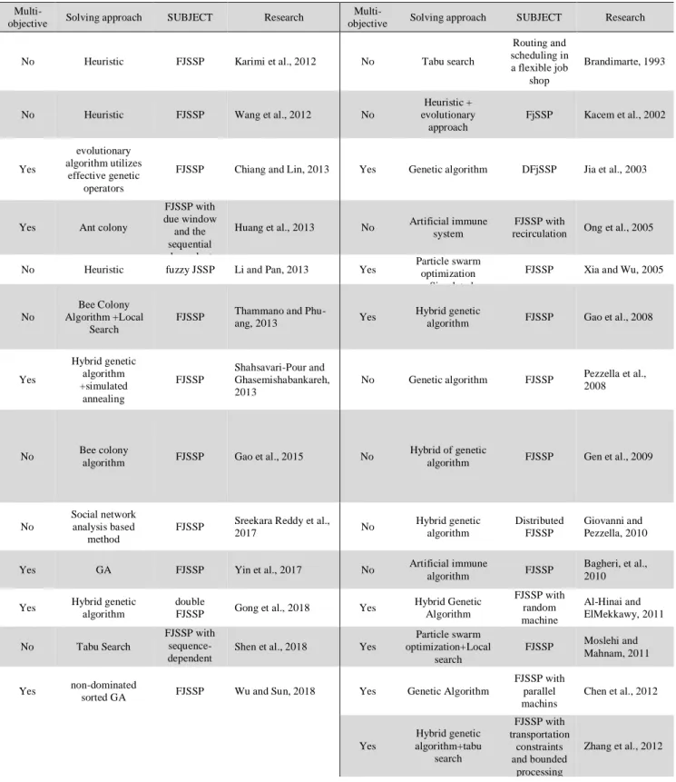
Gong et al. (Gong et al., 2018) proposed a new hybrid genetic algorithm to solve a double FJSSP (DFJSSP) in which both workers and machines are flexible. They presented a multi-objective optimization mathematic model considering the processing time, green production and human factors. Wu and Sun (Wu and Sun, 2018) proposed a non-dominated sorted genetic algorithm to solve FJSSP with Energy-Saving Measures. The objective functions of the problem are minimizing the makespan, the energy consumption and the numbers of turning-on/off machines simultaneously. Many researches in the literature studied flexible job shop scheduling problem. As seen in table 1, some of the researches considered an objective function to the problem and some of them studied multi-objective cases. While some researches added some attributes and constraints to the problem such as sequence-dependent set up times and fuzzy processing times. There are many gaps in the literature of these researches such as lack of other attributes to FJSSP, like orders, ready time and various speeds for machines.

However, some investigations considered the problem without any attributes and focused on developing new solving methods. A glance at the literature shows that the most frequently used algorithm in the literature is genetic algorithm. The other used solving methods are a combination of well-known algorithms such as Tabu search and simulated annealing. This paper adapts RGGA to solve flexible job shop problem with three objective functions: minimizing maximum completion time (Cmax), the maximum machine workload (Wmax), and the total workload (WT).

156

Table 1. Researches’ classification

Multi-objective Solving approach SUBJECT Research

Multi-objective Solving approach SUBJECT Research

No Heuristic FJSSP Karimi et al., 2012 No Tabu search

Routing and scheduling in a flexible job

shop

Brandimarte, 1993

No Heuristic FJSSP Wang et al., 2012 No

Heuristic + evolutionary

approach

FjSSP Kacem et al., 2002

Yes

evolutionary algorithm utilizes

effective genetic operators

FJSSP Chiang and Lin, 2013 Yes Genetic algorithm DFjSSP Jia et al., 2003

Yes Ant colony

FJSSP with due window and the sequential dependent setup time of

jobs

Huang et al., 2013 No Artificial immune system

FJSSP with

recirculation Ong et al., 2005

No Heuristic fuzzy JSSP Li and Pan, 2013 Yes Particle swarm _optimization +Simulated

annealing

FJSSP Xia and Wu, 2005

No

Bee Colony Algorithm +Local

Search

FJSSP Thammano and

Phu-ang, 2013 Yes

Hybrid genetic

algorithm FJSSP Gao et al., 2008

Yes Hybrid genetic algorithm +simulated annealing FJSSP Shahsavari-Pour and Ghasemishabankareh, 2013

No Genetic algorithm FJSSP Pezzella et al., 2008

No Bee colony

algorithm FJSSP Gao et al., 2015 No

Hybrid of genetic

algorithm FJSSP Gen et al., 2009

No

Social network analysis based

method

FJSSP Sreekara Reddy et al.,

2017 No

Hybrid genetic algorithm Distributed FJSSP Giovanni and Pezzella, 2010

Yes GA FJSSP Yin et al., 2017 No Artificial immune _algorithm FJSSP Bagheri, et al., ₂₀₁₀

Yes Hybrid genetic algorithm

double

FJSSP Gong et al., 2018 Yes

Hybrid Genetic Algorithm FJSSP with random machine breakdowns Al-Hinai and ElMekkawy, 2011

No Tabu Search

FJSSP with sequence-dependent setup times

Shen et al., 2018 Yes

Particle swarm optimization+Local

search

FJSSP Moslehi and Mahnam, 2011

Yes non-dominated

sorted GA FJSSP Wu and Sun, 2018 Yes Genetic Algorithm

FJSSP with parallel machins

Chen et al., 2012

Yes Hybrid genetic algorithm+tabu search FJSSP with transportation constraints and bounded processing times

Zhang et al., 2012

3-Research methodology

3-1- Problem description

This paper considers FJSSP. In FJSSP there is a set of jobs J= {J1, ..., Jn} which should be processed by a set of machines S= {M1, ... , Mm}. Each job Ji consists of ni operations Oi1, Oi2,…, Oin, each of which can be processed by a machine. Oik indicates kth operation of job i and could be processed on a set of machines that are shown by Sik, one of them should be selected for processing.

157

Furthermore, it is also assumed that machines in each set may differ in speeds. So, the processing time for each operation may differ on various machines.

Operations should be assigned to a proper machine and sequence of assigned operations to a machine should be determined to minimize three objective functions. The objectives are minimizing maximum completion time (Cmax), the maximum machine workload (Wmax) and the total workload (WT). It is assumed all jobs and machines are available at time zero and preemption is not allowed.

3-2- Research steps

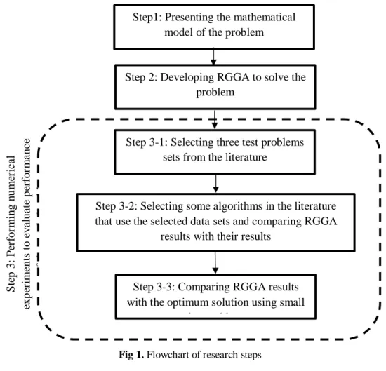
The following steps are performed to solve the problem: Step1: Presenting the mathematical model of the problem.

Step 2: Developing Reference Group Genetic Algorithm (RGGA) to solve the problem. Step 3: Performing numerical experiments to evaluate performance of the used algorithm.

Step 3-1: Selecting three test problems sets from the literature to solve by RGGA(Kacem data set, presented by Kacem et al. (2002), BRdata set presented by Brandimarte (1993) and Fdata proposed by Fattahi et al. (2007).

Step 3-2: Selecting some algorithms in the literature that use the selected data sets and compare RGGA results with their results. (six algorithms using Kacem data set, presented by Kacem et al. (2002). four algorithms using BRdata set presented by Brandimarte (1993), three algorithms using Fdata proposed by Fattahi et al. (2007).) The results of compared algorithms are extracted from their articles.

158

Fig 1. Flowchart of research steps

4- Results

In this section the results of performing research steps are presented.

4-1- Problem formulation

The sets and parameters of the model are as follows: Sets:

Set of n jobs: i=1,2, .., n Set of m machines: j=1,2, .., m

Set of ki operations for job i: k=1, 2, …, ki

Set of

n

available priority positions in machine

j

to process operations:

s=

1, 2, …,

n: number of jobs m: number of machines

ki: number of operations of job i

nj: maximum number of operations that could be assigned to machine j.

Aikj: a zero-one parameter in which Aikj is equal to 1 if Oik can be run on the machine j; else, it is equal to 0.

Pikj: processing time of operation Oik if processed by machine j. L: a sufficiently large number

Also, variables of the model are as follows:

PSik: processing time of operation Oik after choosing a machine. Wj: workload of machine j

Yikj: 1 if machine j is selected to process Oik; otherwise, Yikj = 0. Step1: Presenting the mathematical

model of the problem

Step 2: Developing RGGA to solve the problem

Step 3-1: Selecting three test problems sets from the literature

Step 3-2: Selecting some algorithms in the literature that use the selected data setsand comparing RGGA

results with their results

Step 3-3: Comparing RGGA results with the optimum solution using small

size problems S te p 3 : P er fo rm ing n u m er ic a l exp er im ents t o e v a lua te p er fo rm a nc e o f the us ed a lg o ri thm

159

Xikjs: 1 if Oik runs on machine j with the priority s; otherwise, Xikjs = 0. Tik: start time of processing Oik

TMjs: start time of sth job on machine j.

Pikj is a parameter of the problem and it is the processing time of operation Oik if proceeded by machine j. PSik is a decision variable of the problem and it is processing time of operation Oik after choosing a machine by decision variable Yikj. Finally, the mixed integer mathematical model of the problem is as follows:

Minimize

Z

=

C

Minimize

Z

=

Minimize

Z

= ∑

𝑊

( 1 )

for

i

=1,..,

n

Subject to:

C

≥

T

+ 𝑃𝑆

( 2 )

for

i

=1,..,

n

;

k

=1,..,

k

∑ 𝑌

_𝑖𝑘𝑗

𝑗

×

P

=

PS

( 3 )

for

i

=1,..,

n

;

k

=1,..,

k

-1

T

+PS

_≤

T

( 4 )

for

j

=1,..,

m

;

s=

1,..,

n

-1

TM

+∑

∑

𝑃

×

X

≤

TM

( 5 )

for

j

=1,..,

m

;

s

=1,..,

n

;

i

=1,..,

n

;

k

=1,..,

k

TM

≤

T

+(1−

X

)×

L

( 6 )

for

j

=1,..,

m

;

s

=1,..,

n

;

i

=1,..,

n

;

k

=1,..,

k

TM

+(1−

X

)×

L

≥

T

( 7 )

for

j

=1,..,

m

;

i

=1,..,

n

;

k

=1,..,

k

Y

≤

A

( 8 )

for

i

=1,..,

n

;

k

=1,..,

k

∑ 𝑌

j

=1

( 9 )

for

i

=1,..,

n

;

k

=1,..,

k

∑ ∑ 𝑋

j

=1

( 10 )

for

i

=1,..,

n

;

k

=1,..,

k

j

=1,..,

m

∑ 𝑋

=𝑌

( 11 )

for

j

=1,..,

m

Wj=∑ ∑ 𝑌

×P

( 12 )

for

j

=1,..,

m

W

≥

W

( 13 )

for

j

=1,..,

m

W

for

i

=1,..,

n

;

k

=1,..,

k

T

≥0

for

j

=1,..,

m

;

s

=1,..,

n

;

TM

≥0

for

j

=1,..,

m

;

i

=1,..,

n

;

k

=1,..,

k

Y

∈{0,1}

for

j

=1,..,

m

;

s

=1,..,

n

;

i

=1,..,

n

;

k

=1,..,

k

X

∈{0,1}

Constraint set (1) ensures that Cmax is greater than the completion times of all jobs in the last stage. Constraint set (2) determines processing time of Oik by selecting a machine. Constraint set (3) links

160

the start times of Oik and Oi(k+1). Constraint (4) ensures that no two operations can be performed on the same machine simultaneously. Constraints sets (5) and (6) determine start time of operations assigned to a machine, considering their priority. Constraint set (7) controls ability of machines to process operations. Constraint set (8) guarantees each operation is only assigned to one machine. Constraint set (9) considers any operation only in one priority on its assigned machine. Constraint set (10) explains that an operation does not have any priority on its non-allowable machines. Constraint set (11) determines the workload of each machine. Constraint set (12) determines the maximum machines workload. Constraint set (13) defines type and sign of variables.

4-2- Reference group genetic algorithm

The genetic algorithm is inspired from the natural biological evolution and natural selection. It is used to obtain optimal or near optimal solutions for different problems. The main idea of GAs is to maintain the fittest solutions in order to create better solutions continuously (Zegordi et al., 2010). In this paper, RGGA is adapted to solve the flexible job shop scheduling problem. RGGA employs the role model concept in the sociology to the genetic algorithm.

Sociologist Robert K. Merton hypothesized that individuals compare themselves with reference groups of people who occupy the social role to which the individual aspires (Farazmand and Beheshtinia, 2018). In each society, there are some heroes,professional athletes or celebrities. Heroes are known for some of their characteristics. People in the society try to gain these characteristics named role samples in sociology.

In the society, there are people known as good models and people known as bad models. In the society, people try to match their manner with the good models and make their manner different from bad models. In addition, people’s transactions in the society cause them to influence each other. Humans also try to improve their manner, individually (Najian and Beheshtinia, 2018).

RGGA tries to simulate the process of social evolution. People’s behaviors are promoted by learning from role models, other members of society who are not necessarily role models and by learning from themselves. These three types of learning are implemented in RGGA. The first type is simulated by mutation operators, the second one is implemented by the crossover and the third one is implemented by the individual improvement.

RGGA considers each solution as a chromosome and uses three operators named crossover, mutation and individual improvement to search optimal solution.

4-2-1- Chromosome structure

In the genetic algorithms, each solution is shown as a chromosome. Various coding operators can be employed. In this paper, each chromosome is composed of two strings. The first string determines priority of the whole operation while the second string shows assigned machine for each operation. The first string is composed of several numbers each of which represents an operation of a job. In this string, each job is repeated as the number of its operations.

The second string is as long as the first string and it assigns a machine for each operation. For more explanation, the following example is presented.

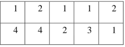
Suppose 2 jobs (J1 and J2) and 4 machines (M1, M2, M3 and M4). The first job has 3 operations and the second job has 2 operations (totally there are 5 operations). A feasible chromosome is shown in figure 2.

2

1

1

2

1

1

3

2

4

4

Fig 2. Chromosome structure

In the first string, the value of the first array is 1. This array represents operation O11. The value of the second array is 2, which represents operation O21. The value of the third array is 1, which represents operations O12.The fourth and fifth arrays represent operations O13 and O22, respectively. The priority of the operations is determined by this string. The string shows O11 has the first priority,

161

O21 has the second one, etc. If two operations are assigned to the same machine, their sequence is determined by its priority.

The second string determines the assigned machine to each operation. In this string, the first array has a value of 4, which indicates O11 should be assigned to machine M4. Also, O21, O12, O13 and O22 should be assigned to M4, M2, M3 and M1.

4-2-2- Initial population

In RGGA, the initial population is randomly generated. Number of chromosomes (pop_size) is one of the RGGA parameters. Fitness value of every chromosome is determined by the objective function. Solutions with better objective function have higher fitness value and vice versa.

The number of chromosomes having the highest fitness value is selected to create a set called Good Role Models (GRM). In addition, a number of chromosomes with the worst fitness value is selected to create a set called Bad Role Models (BRM) set. Size of GRM set (Size good) and BRM set (Size bad) are two parameters of the algorithm.

4-2-3- Reproduction of solutions

RGGA uses crossover, mutation, and individual improvement to search optimal solution of an optimization problem.

The crossover and mutation operators use two procedures, named similarity procedure and dissimilarity procedure. Before describing operators of the algorithm, similarity procedure and dissimilarity procedure are described as follows:

Similarity procedure: Similarity procedure occurs between two chromosomes, one of them as influencer, and the other one as impressible. In similarity procedure some characteristics of impressible are transformed to ones in influencer. Similarity procedure has two phases. In the first phase, the first string of impressible and in the second phase the second string of impressible, are transformed.

In the first string two operations from influencer are selected randomly. Suppose the operations with higher priority as A and the operation with lower priority as B. If priority of B is higher than A in the first string of impressible, then the positions of these operations should be changed in the first string of impressible. Nevertheless, if priority of A is higher than B in the first string of impressible, no changing is required.

In the second phase a random operation is selected and its assigned machine in impressible should be the same as its assigned machine in influencer.

A random integer number (R~U[1, n]) is assigned to impressible, and the mentioned phases are repeated R times. R indicates the degree of acceptance of changes from impressible. If R is small, it means that the impressible has inertia to change it and vice versa.

Dissimilarity procedure: Dissimilarity procedure is occurred between two chromosomes. One of them is assumed as influencer and the other as impressible. In dissimilarity procedure, some characteristics of impressible should be different from ones in influencer. Dissimilarity procedure has two phases. In the first phase, the first string of impressible and in the second phase, the second string of impressible are changed.

In the first string, two operations from influencer are randomly selected. Suppose the operations with higher priority as A and the operation with lower priority as B. If priority of A is higher than B in the first string of impressible, then position of these operations should be changed in the first string of impressible. But if priority of B is higher than A in the first string of impressible, no change is required.

In the second phase, a random operation is selected and its assigned machine in impressible should be different from its assigned machine in influencer.

A random integer number (R~U[1, n]) is assigned to impressible, and the mentioned phases are repeated R times on between influencer and impressible. R indicates the degree of acceptance of changes from impressible. If R is small, it means that the impressible has inertia to change it and vice versa.

After describing similarity and dissimilarity procedure, operators of the algorithm are described as follows:

162

Crossover operator: People in the society are affected by each other. In the crossover operator, two chromosomes are selected randomly. One of them is considered as influencer and the other one is considered as impressible and a similarity procedure is employed.

Number of repetition of the crossover operator is equal to [Cross-rate*pop-size] in which pop-size is the size of initial population and Cross-rate is a Real number between 0 and 1.

Mutation operator: In each society, there are some good models and some bad models. People try to make their characteristics similar to the good models and to make themselves different from the bad models.

The mutation operator is implemented by two steps. In the first step, a chromosome is selected randomly from the current generation as impressible and another chromosome is randomly selected from GRM set, as influencer. Then a similarity procedure is employed.

In the second step a chromosome is randomly selected from BRM set, and it is considered as influencer. Then a dissimilarity procedure is employed.

Number of repetitions of the mutation operator is equal to [Mut-rate*pop-size] in which Mut-rate is a real number between 0 and 1.

Individual improvement: The crossover and mutation operators require chromosomes. In individual improvement operator, members of population try to improve themselves independently. In Individual improvement operator, a chromosome is selected at random and is changed in two steps. In the first step, two arrays in the first string are selected randomly and their values swapped. In the second step, an operation is randomly selected and its assigned machine is changed to another one.

Number of repetition of the individual improvement operator is one of the RGGA parameters and is represented by the notation r.

4-2-4- Other algorithm operators

In RGGA, chromosomes are selected randomly for crossover and mutation operators. But to select the chromosomes for the next population, RGGA uses elitism and roulette wheel methods. For this purpose, [BEST*pop-size] chromosomes having better fitness value are selected for the next population and the remaining pop-size -[BEST*pop-size] chromosomes are selected based on roulette wheel method. The value of BEST parameter is between 0 and 1. Moreover, if the best founded chromosome of population does not improve in the Max-iter consecutive generation, the algorithm is terminated.

After various runs, it is empirically found that the value of 100 for pop-size, 5 for Size_good and Size_bad, 0.2 for Cross_rate, 0.6 for Mut_rate, 0.1 for r, 0.1 for BEST and 10 for Max-iter gives good results in a reasonable CPU time.

4-3- Numerical experiments

In this section, the performance of RGGA is evaluated by comparing it with other algorithms that have been proposed in the literature. The algorithm is coded in Matlab and was implemented on an Intel Core i7-7700 PC.

4-3-1- Test data

In this paper, three standard test data sets available in the literature are used as follow:

(1) Kacem data: This data set is a set of three problems (problem 8×8, problem 10×10 and problem 15×10) (Kacem et al., 2002). Problem 8×8 is an instance of partial flexibility that consists of 8 jobs with 27 operations which can be processed on 8 machines, Problem10×10 has total flexibility that consists of 10 jobs with 30 operations which can be implemented on 10 machines, and Problem 15×10 has total flexibility that consists of 15 jobs with 56 operations which can be performed on 10 machines. The details about Kacem data can be found in Xia and Wu (2005).

(2) BRdata: This data set consists of 10 test problems from Brandimarte (1993). The number of jobs was determined according to the uniform distribution U[10, 20]; the number of machines followed the uniform distribution U[4, 15], the number of operations for each job matched the uniform distribution U[5, 15], and the number of operations for all jobs followed the uniform distribution U[55, 240].

163

(3) Fadata: The data set consists of 20 test problems proposed by Fattahi et al. (2007). These test problems are divided to two categories: small size flexible job-shop scheduling problems (SFJS1:10), and medium and large size flexible job-shop scheduling problems (MFJS1:10). The number of jobs ranges from 2 to 12, the number of machines ranges from 2 to 8, the number of operations for each job ranges from 2 to 4, and the number of operations for all jobs ranges from 4 to 48.

4-3-2- Experiment results

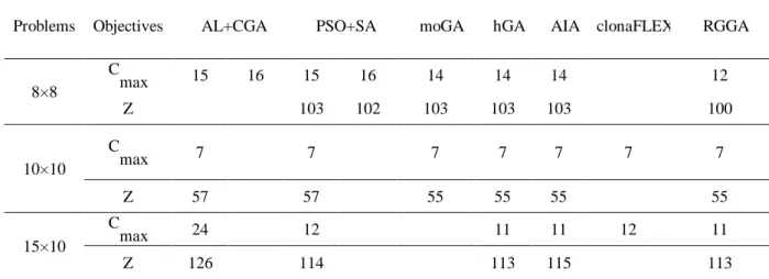
In this section results of RGGA is compared with various algorithms in the literature. The results of compared algorithms are extracted from their articles and they are not run in this research. In table 2, RGGA is compared to AL+CGA proposed by Kacem et al. (2002), PSO+SA proposed by Xia and Wu (2005), a multistage operation-based GA (moGA) proposed by Gen et al. (2009), a clonal selection based algorithm (ClonaFLEX) proposed by Ong et al. (2005), an Artificial Immune Algorithm (AIA) proposed by Bagheri et al. (2010) and a hybrid Genetic Algorithm (hGA) proposed by Gao et al. (2008). The results reveal RGGA outperforms other algorithms. All mentioned algorithms used Kacem data and their results are shown in table 2 in which Z refers to sum of all tree objective functions. Some cells in table 2 are empty because the mentioned papers do not consider the related objective function or the results are not presented in the papers.

Table 2. Results on Kacem data

Problems Objectives AL+CGA PSO+SA moGA hGA AIA clonaFLEX RGGA

8×8

C

max 15 16 15 16 14 14 14 12

Z 103 102 103 103 103 100

10×10 C

max 7 7 7 7 7 7 7

Z 57 57 55 55 55 55

15×10 C

max 24 12 11 11 12 11

Z 126 114 113 115 113

The first algorithm examined in table 2 is AL + CGA algorithm by Kacem et al. (2002). They solved partial 8×8 flexible job shop by Approach Localization (AL) and a genetic algorithm named CGA. They present two solutions to this problem. The first solution (Cmax =15) is obtained by an algorithm which uses a combination of AL and CGA (AL+CGA). The second solution (Cmax =16) is obtained by an algorithm which uses only localization approach. 10×10 and 15×10 problems are solved by AL+CGA.

The second algorithm in table 2 is provided by the Xia and Wu (2005). This algorithm is a Partial Swarm Optimization (PSO) algorithm which uses a Simulated Annealing (SA) approach as a sub-algorithm (PSO+SA). Indeed, each particle’s fitness value in PSO is computed by SA sub-algorithm. Xia and Wu (2005) and Gen et al. (2009) present two solutions for partial 8×8 flexible job shop. The first solution (Cmax =15 and Z=103) has better value for Cmax, but the second one (Cmax =16 and and Z=102) has better value for Z. For 10×10 and 15×10 problems, only one solution is presented. RGGA provides value of 11 for Cmax and value of 100 for Z for 8×8 problem and outperforms other algorithms.

All the algorithms provide value 7 for Cmax in 10×10 problem. In this case, RGGA has better results than AL+CGA and PSO+SA. In 10×15 problem, RGGA has better value for Cmax than AL+CGA, PSO+SA, clonaFLEX. In this case RGGA has better value for Z than other algorithms except hGA. The second data set used for comparison is BRdata data set which is provided by Brandimarte (1993). This test data set contains 10 different problems.

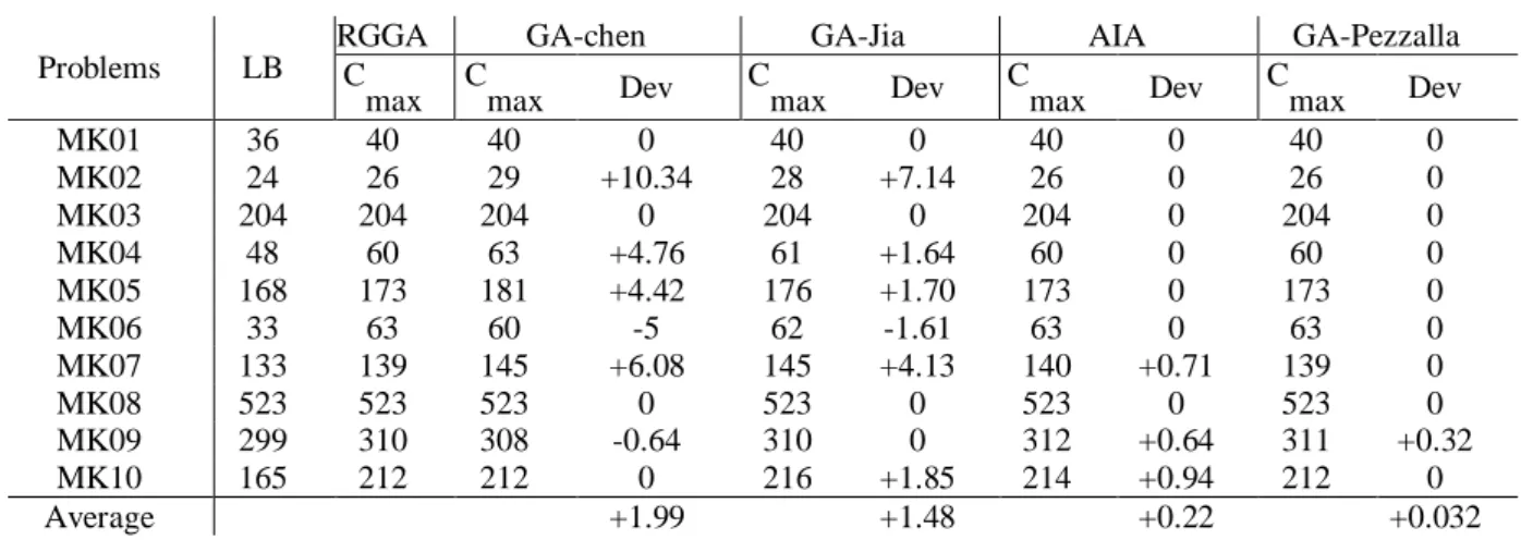
Table 3 compares RGGA beside four algorithms in the literature including three genetic algorithms, GA-chen, proposed by Chen et al. (2012); GA-Jia proposed by Jia et al. (2003); GA-Pezzalla

164

proposed by Pezzella et al. (2008), and an artificial immune system (AIA) proposed by Bagheri et al. (2010). Table 3 only considers Cmax objective function, because the mentioned papers do not consider other objective functions or do not preset its result on BRdata.

To compare RGGA with other algorithms, a criterion introduced by Bagheri et al. (2010) is employed. The relative deviation is defined as

𝐷𝑒𝑣 = [(𝐶

− 𝐶

)/𝐶

] ∗ 100%

Where Cbest is the makespan obtained by the RGGA and Cf is the makespan of compared algorithm. A positive value of Dev indicates the superiority of RGGA in comparison to other algorithms and vice versa. In table 3, the mean on Dev is positive. This indicates RGGA presents overall better results in comparison with the other algorithms.

Table 3. Results on Brdata

Problems LB

RGGA GA-chen GA-Jia AIA GA-Pezzalla

C

max Cmax Dev Cmax Dev Cmax Dev Cmax Dev

MK01 36 40 40 0 40 0 40 0 40 0

MK02 24 26 29 +10.34 28 +7.14 26 0 26 0

MK03 204 204 204 0 204 0 204 0 204 0

MK04 48 60 63 +4.76 61 +1.64 60 0 60 0

MK05 168 173 181 +4.42 176 +1.70 173 0 173 0

MK06 33 63 60 -5 62 -1.61 63 0 63 0

MK07 133 139 145 +6.08 145 +4.13 140 +0.71 139 0

MK08 523 523 523 0 523 0 523 0 523 0

MK09 299 310 308 -0.64 310 0 312 +0.64 311 +0.32

MK10 165 212 212 0 216 +1.85 214 +0.94 212 0

Average +1.99 +1.48 +0.22 +0.032

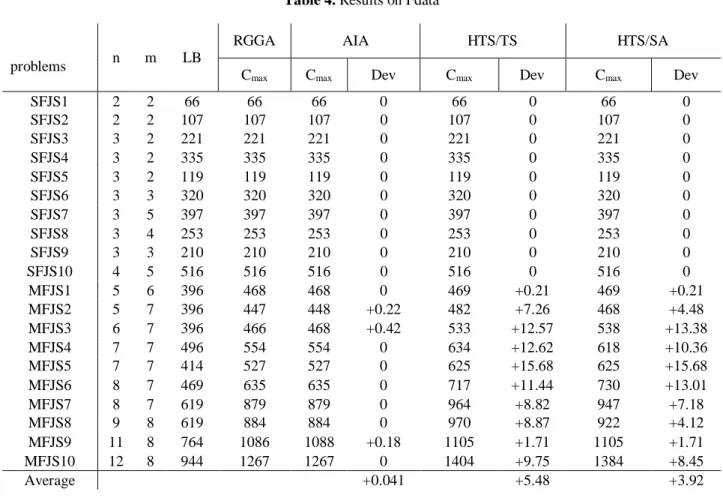
In table 4, based on Fdata data set, RGGA is compared to hierarchical approaches, namely HTS/TS and HTS/SA algorithms proposed by Fattahi et al. (2007) and AIA proposed by Bagheri et al. (2010). In table 4, the mean on Dev is positive. This implies RGGA presents overall better results in comparison with the other algorithms.

165

Table 4. Results on Fdata

problems n m LB

RGGA AIA HTS/TS HTS/SA

Cmax Cmax Dev Cmax Dev Cmax Dev

SFJS1 2 2 66 66 66 0 66 0 66 0

SFJS2 2 2 107 107 107 0 107 0 107 0

SFJS3 3 2 221 221 221 0 221 0 221 0

SFJS4 3 2 335 335 335 0 335 0 335 0

SFJS5 3 2 119 119 119 0 119 0 119 0

SFJS6 3 3 320 320 320 0 320 0 320 0

SFJS7 3 5 397 397 397 0 397 0 397 0

SFJS8 3 4 253 253 253 0 253 0 253 0

SFJS9 3 3 210 210 210 0 210 0 210 0

SFJS10 4 5 516 516 516 0 516 0 516 0

MFJS1 5 6 396 468 468 0 469 +0.21 469 +0.21

MFJS2 5 7 396 447 448 +0.22 482 +7.26 468 +4.48

MFJS3 6 7 396 466 468 +0.42 533 +12.57 538 +13.38

MFJS4 7 7 496 554 554 0 634 +12.62 618 +10.36

MFJS5 7 7 414 527 527 0 625 +15.68 625 +15.68

MFJS6 8 7 469 635 635 0 717 +11.44 730 +13.01

MFJS7 8 7 619 879 879 0 964 +8.82 947 +7.18

MFJS8 9 8 619 884 884 0 970 +8.87 922 +4.12

MFJS9 11 8 764 1086 1088 +0.18 1105 +1.71 1105 +1.71

MFJS10 12 8 944 1267 1267 0 1404 +9.75 1384 +8.45

Average +0.041 +5.48 +3.92

Table 5 compares the results of RGGA with the optimum solution using 10 random small size problems. In this table each problem is shown by two numbers. The first number is the number of orders and the second one is the number of machines. The optimum solution is obtained by Lingo 8 software. Since our problem is a multi-objective function, a linear combination of the objectives is used considering a weight equal to 1/3 for each objective function. Results show that when the size of the problem is small, RGGA obtains an approximately optimum solution. Also, the CPU time of the RGGA is less than CPU time of LINGO software.

Table 5. Comparison of RGGA and optimum solution

RGGA Optimum

Problem size Solution CPU

time Solution

CPU

time dev

3×2 26 2 26 11 0

4×2 26.333 2 26.333 8 0

5×2 43 3 42 169 0.023256

3×3 25.333 2 25.333 46 0

4×3 28.667 2 28.667 19 0

5×3 40.333 3 39.333 1884 0.024793

3×4 31.333 2 31.333 43 0

4×4 34.333 5 34.333 201 0

5×4 57 5 56.83 444 0.002982

166

5- Discussion and conclusion

In this research, a flexible job shop scheduling problem with minimizing three objective functions containing the maximum completion times of jobs (Cmax), the maximum machine workload (Wmax) and the total workload (WT) is investigated.

After presenting the mathematical model of the problem, RGGA based on the role model concept in the sociology is adapted to solve the problem.

Various researches try to employ some characters of various phenomena in optimization algorithms (Beheshtinia and Ghasemi, 2018). Genetic algorithm is a frequently used optimization algorithm and various researches try to add some characters to it or combine it with another algorithm to enhance its performance (Borumand and Beheshtinia). A glance at the history shows that the social evolution is very faster than the genetic evolution. Classical genetic algorithms simulate the genetic evolution. Identifying the characters of social evolution and employing them to an algorithm may causes better results. One of these characters is the concept of role models introduced by sociologist Robert K. Merton. Two types of role models called good role models and bad role models are defined. People try to make themselves similar to good models and different from bad models.

Comparison of RGGA with genetic algorithm shows that:

 In RGGA, the best and the worst obtained solutions are saved in GRM and BRM sets respectively. But this information in GA is not saved.

 In the genetic algorithm, the output of mutation operator is a solution that inherits characters from one solution, while in RGGA the output of mutation operator is a solution that inherits the characters from three other solutions: a random solution from the current population, a good role model and a bad role model.

 The crossover operator in RGGA is based on similarity procedure and a parent tries to imitate some characters from another one and vice versa. In other words, the overall structure of the parent is kept and some of its characters are changed based on the other parent. While in GA the parents are mixed randomly.

The results of numerical experiments demonstrate the acceptable performance of the RGGA. The most critical aspect of the RGGA is its mutation operator. Good role models have better fitness function in comparison with other chromosomes, so they have some desirable attributes. In the first phase of the mutation operator, RGGA tries to convey these desirable attributes from the good role model to the population. This procedure enhances the quality of the population. On the other hand, bad role models have some undesirable attributes. In the second phase of the mutation operator, RGGA tries to eliminate these undesirable attributes from the population. This procedure also enhances the population’s quality.

In the future, it can be interesting to develop other versions of RGGA such as considering other individual improvement operators or other similarity procedures. Merging RGGA with other heuristics and meta-heuristics may be another possibility for future research. Moreover, the use of RGGA to other problems and evaluating its performance on various scopes of optimization problems can be a promising research direction.

References

Abdelmaguid, T. F. (2015). A neighborhood search function for flexible job shop scheduling with separable sequence-dependent setup times. Applied Mathematics and Computation, 260,188-203. Al-Hinai, N., &ElMekkawy, T. Y. (2011). Robust and stable flexible job shop scheduling with random machine breakdowns using a hybrid genetic algorithm. International Journal of Production Economics, 132(2), 279-291.

Bagheri, A., Zandieh, M., Mahdavi, I., &Yazdani, M. (2010). An artificial immune algorithm for the flexible job-shop scheduling problem. Future Generation Computer Systems, 26(4), 533-541.

167

Beheshtinia, M. A., &Ghasemi, A. (2018). A multi-objective and integrated model for supply chain scheduling optimization in a multi-site manufacturing system. Engineering Optimization, 50(9), 1415-1433.

Beheshtinia, M. A., Ghasemi, A., &Farokhnia, M. (2018). Supply chain scheduling and routing in multi-site manufacturing system (case study: a drug manufacturing company). Journal of Modelling in Management, 13(1), 27-49.

Borumand, A., & Beheshtinia, M. A. (2018). A developed genetic algorithm for solving the multi-objective supply chain scheduling problem. Kybernetes.

Bożejko, W., Uchroński, M., &Wodecki, M. (2010). Parallel hybrid metaheuristics for the flexible job shop problem. Computers & Industrial Engineering, 59(2), 323-333.

Brandimarte, P. (1993). Routing and scheduling in a flexible job shop by tabu search. Annals of Operations Research, 41(3), 157-183.

Chen, J. C., Wu, C.-C., Chen, C.-W., &Chen, K.-H. (2012). Flexible job shop scheduling with parallel machines using Genetic Algorithm and Grouping Genetic Algorithm. Expert Systems with Applications, 39(11), 10016-10021.

Chiang, T.-C., &Lin, H.-J. (2013). A simple and effective evolutionary algorithm for multiobjective flexible job shop scheduling. International Journal of Production Economics, 141(1), 87-98.

De Giovanni, L., &Pezzella, F. (2010). An Improved Genetic Algorithm for the Distributed and Flexible Job-shop Scheduling problem. European Journal of Operational Research, 200(2), 395-408.

Farazmand, N., & Beheshtinia, M. (2018). Multi-objective optimization of time-cost-quality-carbon dioxide emission-plan robustness in construction projects. Journal of Industrial and Systems Engineering, 11(3), 102-125.

Fattahi, P., Saidi Mehrabad, M., &Jolai, F. (2007). Mathematical modeling and heuristic approaches to flexible job shop scheduling problems. Journal of Intelligent Manufacturing, 18(3), 331-342.

Gao, J., Sun, L., &Gen, M. (2008). A hybrid genetic and variable neighborhood descent algorithm for flexible job shop scheduling problems. Computers & Operations Research, 35(9), 2892-2907.

Gen, M., Gao, J., & Lin, L. (2009). Multistage-based genetic algorithm for flexible job-shop scheduling problem. In Intelligent and evolutionary systems (pp. 183-196). Springer, Berlin, Heidelberg.

Gong, G., Deng, Q., Gong, X., Liu, W., &Ren, Q. (2018). A new double flexible job-shop scheduling problem integrating processing time, green production, and human factor indicators. Journal of Cleaner Production, 174,560-576.

Huang, R.-H., Yang, C.-L., &Cheng, W.-C. (2013). Flexible job shop scheduling with due window— a two-pheromone ant colony approach. International Journal of Production Economics, 141(2), 685-697.

Jia, H. Z., Nee, A. Y. C., Fuh, J. Y. H., &Zhang, Y. F. (2003). A modified genetic algorithm for distributed scheduling problems. Journal of Intelligent Manufacturing, 14(3/4), 351-362.

Kacem, I., Hammadi, S., &Borne, P. (2002). Approach by localization and multiobjective

evolutionary optimization for flexible job-shop scheduling problems. Systems, Man, and Cybernetics, Part C: Applications and Reviews, IEEE Transactions on, 32(1), 1-13.

168

Kaplanoğlu, V. (2016). An object-oriented approach for multi-objective flexible job-shop scheduling problem. Expert Systems with Applications, 45, 71-84.

Karimi, H., Rahmati, S. H. A., &Zandieh, M. (2012). An efficient knowledge-based algorithm for the flexible job shop scheduling problem. Knowledge-Based Systems, 36,236-244.

Li, J.-q., &Pan, Q.-k. (2013). Chemical-reaction optimization for solving fuzzy job-shop scheduling problem with flexible maintenance activities. International Journal of Production Economics, 145(1),

4-17.

Liu, B., Fan, Y., &Liu, Y. (2015). A fast estimation of distribution algorithm for dynamic fuzzy flexible job-shop scheduling problem. Computers & Industrial Engineering, 87,193-201.

Merton, R. K., & Barber, E. (2011). The travels and adventures of serendipity: A study in sociological semantics and the sociology of science. Princeton University Press.

Moslehi, G., &Mahnam, M. (2011). A Pareto approach to multi-objective flexible job-shop scheduling problem using particle swarm optimization and local search. International Journal of Production Economics, 129(1), 14-22.

Najian, M. H., & Beheshtinia, M. A. (2018). Supply Chain Scheduling Using a Transportation System Composed of Vehicle Routing Problem and Cross-Docking Approaches. International Journal of Transportation Engineering.

Ong, Z. X., Tay, J. C., &Kwoh, C. K. (2005). Applying the Clonal Selection Principle to Find Flexible Job-Shop Schedules. Artificial Immune Systems. Springer Berlin Heidelberg.

Pezzella, F., Morganti, G., &Ciaschetti, G. (2008). A genetic algorithm for the Flexible Job-shop Scheduling Problem. Computers & Operations Research, 35(10), 3202-3212.

Shahsavari-Pour, N., &Ghasemishabankareh, B. (2013). A novel hybrid meta-heuristic algorithm for solving multi objective flexible job shop scheduling. Journal of Manufacturing Systems, 32(4), 771-780.

Shen, L., Dauzère-Pérès, S., &Neufeld, J. S. (2018). Solving the flexible job shop scheduling problem with sequence-dependent setup times. European Journal of Operational Research, 265(2),

503-516.

Shi-Jin, W., Bing-Hai, Z., &Li-Feng, X. (2008). A filtered-beam-search-based heuristic algorithm for flexible job-shop scheduling problem. International Journal of Production Research, 46(11), 3027-3058.

Sreekara Reddy, M. B. S., Ratnam, C. h., Agrawal, R., Varela, M. L. R., Sharma, I., &Manupati, V. K. (2017). Investigation of reconfiguration effect on makespan with social network method for flexible job shop scheduling problem. Computers & Industrial Engineering, 110, 231-241. Tang, J., Zhang, G., Lin, B., &Zhang, B. (2011). A Hybrid Algorithm for Flexible Job-Shop Scheduling Problem. Procedia Engineering, 15, 3678-3683.

Thammano, A., &Phu-ang, A. (2013). A Hybrid Artificial Bee Colony Algorithm with Local Search for Flexible Job-shop Scheduling Problem. Procedia Computer Science, 20, 96-101.

Wang, L., Wang, S., Xu, Y., Zhou, G., &Liu, M. (2012). A bi-population based estimation of distribution algorithm for the flexible job-shop scheduling problem. Computers & Industrial Engineering, 62(4), 917-926.

169

Wu, X., &Sun, Y. (2018). A green scheduling algorithm for flexible job shop with energy-saving measures. Journal of Cleaner Production, 172, 3249-3264.

Xia, W., &Wu, Z. (2005). An effective hybrid optimization approach for multi-objective flexible job-shop scheduling problems. Computers & Industrial Engineering, 48(2), 409-425.

Yin, L., Li, X., Gao, L., Lu, C., &Zhang, Z. (2017). A novel mathematical model and multi-objective method for the low-carbon flexible job shop scheduling problem. Sustainable Computing: Informatics and Systems, 13, 15-30.

Zegordi, S. H., Abadi, I. N. K., &Nia, M. A. B. (2010). A novel genetic algorithm for solving production and transportation scheduling in a two-stage supply chain. Computers & Industrial Engineering, 58(3), 373-381.

Zhang, Q., Manier, H., &Manier, M. A. (2012). A genetic algorithm with tabu search procedure for flexible job shop scheduling with transportation constraints and bounded processing times. Computers & Operations Research, 39(7), 1713-1723.