A Goal Programming Method for Finding Common Weights in DEA with an Improved Discriminating Power for Efficiency

Winter 2008

A Goal Programming Method for Finding Common Weights in DEA with

an Improved Discriminating Power for Efficiency

A. Makui1∗, A. Alinezhad2, R. Kiani Mavi3,M. Zohrehbandian4

1

Department of Industrial Engineering, Iran University of Science & Technology, Tehran, Iran. (E-mail: [email protected]

2,3

Department of Industrial Engineering, Islamic Azad University-Science & Research Branch, Tehran, Iran. [email protected]

[email protected]

4

Department of Mathematics, Islamic Azad University-Karaj P.O.Box 31485-313, Karaj, Iran. [email protected]

ABSTRACT

A characteristic of data envelopment analysis (DEA) is to allow individual decision making units (DMUs) to select the most advantageous weights in calculating their efficiency scores. This flexibility, on the other hand, deters the comparison among DMUs on a common base. For dealing with this difficulty and assessing all the DMUs on the same scale, this paper proposes using a multiple objective linear programming (MOLP) approach for generating a common set of weights in the DEA framework.

Keywords: MOLP, Goal programming, DEA, Efficiency, Ranking, Weight restrictions. 1. INTRODUCTION

Data envelopment analysis (DEA) has been widely applied to measure the relative efficiency of a group of homogeneous decision making units (DMUs) with multiple inputs and multiple outputs. Its characteristic is to focus on each individual DMU to select the weights attached to the inputs and outputs, and to calculate their efficiency scores.

As the mathematical models in DEA are run separately for each DMU, the set of weights will be different for the various DMUs, and in some cases, it is unacceptable that the same factor is accorded widely differing weights. This flexibility in selecting the weights, deters the comparison among DMUs on a common base. A possible answer to this difficulty lies in the specification of a common set of weights, which was first introduced by Roll et al.(1991). In other words, the major purpose for generating a common set of weights is to provide a common base for ranking the DMUs.

Research on the idea of a common set of weights and their rankings has grown gradually in recent years. Kao and Hung (2005), based on multiple objective nonlinear programming and by using

∗

compromise solution approach, proposed a method to generate a common set of weights for all DMUs which are able to produce a vector of efficiency scores closest to the efficiency scores calculated from the standard DEA model (ideal solution). Likewise, Jahanshahloo et al.(2005) based on multiple objective nonlinear programming and Maximization of the minimum value of the efficiency scores, proposed a method to generate a common set of weights for all DMUs. Some of the other studies in this field are attributed to Doyle and Green (1994), Karsak and Ahiska (2005), Roll and Golany (1993).

The plan for the rest of this paper is as follows. In section 2 we present a brief discussion about DEA models and the multiple objective linear programming (MOLP). The mathematical foundation of our method for finding a common set of weights and the method itself are discussed in Section 3. A Numerical example is presented in section 4 and finally, section 5 draws the conclusive remarks.

2. DEA AND MOLP PRELIMINARIES

Thirty years after the publication of the pioneering paper by Charnes et al.(1978), DEA can safely be considered as one of the recent success stories in Operations Research. Interestingly, Charnes and Cooper have also developed Goal Programming (GP) that is a multiple objective linear programming technique (Charnes and Cooper, 1961). Since the 1970s, MOLP has become a popular approach for modeling and analyzing certain types of multiple criteria decision making (MCDM) problems. Some work on the interactions between MCDM and DEA, are as follows: Bouyssou (1999), Estellita et al.(2004), Giokas (1997), Golany (1988), Joro et al.(1998), Stewart (1996), and Xiao and Reeves (1999).

Data Envelopment Analysis

Consider n production units, or DMUs, each of which consumes a varying amount of m inputs to produce s outputs. Suppose

_x

_ij≥0denotes the amount consumed by the ith input and

y

≥

0

rj

denotes the amount produced by the rth output for the jth decision making unit. Then, the following set is the production possibility set (PPS) of obviously the most widely used DEA model, CCR, with constant returns to scale characteristics:

( )

⎭ ⎬ ⎫ ⎩

⎨ ⎧

= ≥

≤ ≥

= x y x

∑

₌ y

∑

n_{= j} j n

j j j

n

j j j

c

x

y

T

, , , 0, 1,2,...,

1

1

λ

λ

λ

Definition 1:

_DMU

_j

,

j

=

1

,

2

,...,

n

is called efficient iff there does not exist another

( )

x

,

y

∈

T

csuch that

x

<

x

jand

y

>

y

_j, and is called Pareto efficient iff there does not exist

another

( )

x

,

y

∈

_T

_csuch that

x

≤

_x

_j and

y

≥

y

_j and

( )

x

,

y

≠

(

_x

_j

,

y

_j

)

.

In DEA, the measure of efficiency of a DMU is defined as a ratio of a weighted sum of outputs to a weighted sum of inputs subject to the condition that corresponding ratios for each DMU are less than or equal to one. The model chooses nonnegative weights for a DMU in a most favorable way. The original model proposed by Charnes et al.(1978), for measuring the efficiency of unit ’p’, is a fractional linear program as follows:

∑

∑ (1)

subject to ∑

∑ 1

1,2,

,

0

1,2,

,

0 1,2, ,

where

_u

_r and

_v

_iare the weights to be applied to the outputs and inputs, respectively.

The above model can be transformed to a linear program by setting the denominator in the objective function equal to an arbitrary constant (e.g., unity) and maximizing the numerator. The resulting model, called an input oriented CCR multiplier model (CCRm), is as follows:

1

1 1

1 )

0, 1, 2,...,

1

0, 1, 2,..., 0, 1, 2,...,

s

m r r rp

s m

ij

r i

r rj i

m

ip i i

r i

CCR Max

subject to

j n

r s

i m

y

u

y

u

v x

v x

u

v

=

= =

=

− ≤ =

=

≥ =

≥ =

∑

∑

∑

∑

(2)

The optimum solution of the problem is associated to a normalized coefficient

(

−

_v

*

,

_u

*

)

of a supporting hyperplane (a hyperplane that contains the PPS in only one of the halfspaces and passes through at least one of its points). The dual problem of CCRm model called input oriented CCR envelopment model (CCRe), will also be used. This model has a strong intuitive appeal and is

typically the one used to explain and visualize DEA. If θp represents the CCR efficiency of DMUp

then the CCRe model is

1

1 )

0, 1, 2,...,

, 1, 2,...,

0, 1, 2,...,

e p

n

ij ip

j p

j n

j

j rj rp

j

CCR Min

subject to

i m

r s

j n

x

x

y

y

θ

λ

θ

λ

λ

=

=

− ≤ =

≥ =

≥ =

∑

∑

(3)

A DMU is efficient if and only if the objective function value associated with the optimal solution of the problem (1) above equals to unity; otherwise it is inefficient. Moreover, if in the former model all variables take a strictly positive value or as in its counterpart in the latter model all slack variables are equal to zero, the DMU is Pareto efficient. According to Kao and Hung (2005) and based on the solution of model (3), we present the following lemmas.

Lemma 1: If

θ

*_p is the optimum solution of model (3), then

(

θ

*_p

_x

_p

,

y

_p

)

, called projection of DMUp on the efficient frontier, is an efficient virtual DMU.

Lemma 2: DMUp is efficient iff there exist a nonnegative coefficient

( )

R

R

s m

u

v

,

∈

×

associated to the gradient vector of a supporting hyperplane where we have:

0

1

1

−

∑

=

∑

= mi= i ip

s

r

u

r

y

rp

v

x

We now present a brief introduction of MOLP

Multiple Objective Linear Programming

The MOLP problem can be written in the general form as follows:

{

}

( ) :

( ) 0, 1, 2,...,

i

Max f x Cx

subject to

x X x

g

x i m

=

∈ = ≤ =

(4)

Where

x

∈

_R

n, the objective function matrix

C

∈

_R

k×n and

g

_i

(

x

)

≤

0

,

i

=

1

,

2

,...,

m

, are linear functions.

In MOLP, an efficient solution is introduced as follows:

Definition 2:

_x

*

∈

X

is called an efficient solution (or non-dominated solution) iff there does not exist another

x

∈

X

such that

_Cx

≥

_Cx

*and

_Cx

≠

_Cx

*.

In order to solve model (4) and identifying the efficient solutions, there are many different methods in the literature. One of these methods is Goal Programming which is developed by Charnes and Cooper (1961). This method requires the decision maker (DM) to set goals for each objective that he/she wishes to attain. A preferred solution is then defined as the one which minimizes the deviations from the set of goals. Thus a simple GP formulation is given by:

(

)

1

1

, 1

. :

( ) 0 1, 2,...,

( ) 1, 2,...,

, 0 1, 2,...,

0 1, 2,...,

k p p

j j

j

i

j j j j

j j

j j

Min p

S T

x i m

x j k

j k

j k

d

d

g

d

d

b

f

d d

d

d

− +

=

− +

− +

− +

⎡ ⎤

+ ≥

⎢ ⎥

⎣ ⎦

≤ =

+ − = =

≥ =

× = =

∑

Where fj, j = 1, … , k are objectives;

b

_j , j=1,...,k are the goals set by the DM for the objectives,

d

j

−

and

_d

+_jare the under-achievement and over-achievement of the jth goal respectively . The value of p is based upon the utility function of the DM.

Now, by combining DEA and MOLP we present a new method for finding a common set of weights.

3. A METHOD FOR FINDING A COMMON SET OF WEIGHTS

Kornbluth (1991) noticed that the DEA model could be expressed as a multi-objective linear fractional programming problem. The objective function of the model is the same as in the CCR model (1) which attempts to maximize the efficiency of all DMUs collectively, instead of one at a time by the same constraints. However, the proposed model is nonlinear. Based on Kornbluth’s approach some other methods also have been proposed in the literature, all of which are nonlinear. In this section, we present an improvement to Kornbluth’s approach by introducing an MOLP for finding common weights in DEA. The following model which provides the same results as the CCR multiplier model is introduced to find the efficiency value of DMUp. This model has some

advantages compared to foregoing models that will be discussed later.

(

)

(

)

*

1 1

*

1 1

1 1

0, 1, 2,...,

1

0, 1, 2,..., 0, 1, 2,...,

s m

ip

r p i

r rp i

s m

ij

r j i

r rj i

s m

r i

r i

r i

Max subject to

j n

r s

i m

y

u

v x

y

u

v x

u

v

u

v

θ

θ

= =

= =

= =

−

− ≤ =

+ =

≥ =

≥ =

∑

∑

∑

∑

∑

∑

(6)

Where

θ

*_j

,

j

=

1

,

2

,...,

n

is the optimum value obtained from the CCRe model, when DMUj is

under consideration.

We present the following theorem to address the optimal solution of the model in (6).

Theorem 1: The optimum value of the model in (6) is zero and for its optimal solution, say

(

u

*

,

v

*

)

, we have

θ

*

1 * 1

*

p m

i i ip s

r r rp

x

v

y

u

=

∑

∑

= =

.

Proof : Since

(

_x

_y

)

p p p

,

*

θ

is input oriented projection of DMUp on the efficient frontier, hence it

According to the above model and the proposed approach by Kornbluth (1991), The idea behind the identification of the common weights is formulated as the maximizing the ratio of outputs to inputs for all projected DMUs simultaneously. So we present the following MOLP problem.

* *

1 1

1 1 1 1 1

*

1 1

1 1

,...,

0, 1, 2,...,

1

0, 1, 2,..., 0, 1, 2,...,

s m s m

i in

r i r i n

r r i r rn i

s m

ij

r i j

r rj i

s m r i r i r i Max subject to j n r s i m

y

y

u

v

x

u

v

x

y

u

v

x

u

v

u

v

θ

θ

θ

= = = = = = = = ⎡ _{− −} ⎤ ⎣ ⎦ − ≤ = + = ≥ = ≥ =

∑

∑

∑

∑

∑

∑

∑

∑

(7)

Furthermore, in order to solve the above MOLP model, we set p=1 and use a goal programming with all goals equal to zero.

(

)

1 * 1 1 * 1 1 1 1

0, 1, 2,...,

0, 1, 2,...,

1

, 0, 1, 2,..., 0, 1, 2,..., 0, 1, 2,...,

n

j j

j

s m

ij

r i j

r rj i

s m

ij

r i j j j

r rj i

s m r i r i j j r i Min subject to j n j n j n r s i m

d

d

y

u

v

x

y

u

v

x

d

d

u

v

d d

u

v

θ

θ

− + = = = − + = = = = − + + − ≤ = − + − = = + = ≥ = ≥ = ≥ =

∑

∑

∑

∑

∑

∑

∑

(8)

Here, due to the fact that p=1 and model is linear, the last set of constraints in model (5) does not appear in the above model. Moreover, the first and the second set of constraints in model (8) force

d

j

+

to take value zero. However, solving the above GP model gives us a common set of weights and then the efficiency scores of DMUj , j=1,...,n, can be obtained by using these common weights

as

∑

∑

= = m

i i ij s

r r rj

x

v

y

u

1 * 1 *

. If for

(

_u

*

,

_v

*

)

we have

1

1 * 1 *

=

∑

∑

= = m

i i ij s

r r rj

x

v

y

u

, then DMUp is called efficient.

Based on the work of Kao and Hung (2005) we can propose the following lemma.

Lemma 3: A DMUp which is shown to be efficient by model (8), also is efficient in the input

oriented CCR model.

Theorem 2: There exists a DMUj , j=1,...,n which is characterized as the efficient DMU by

model (8).

Proof:. There is a DMUp,

p

∈

{

1

,

2

,...,

n

}

for which the first inequality in (8) is binding. Because,

if that is not the case, there exists a sufficiently small value

ε

>

0

for which

( )

u

,

v

=

(

_u

*

+

[

ε

,

0

,...,

0

]

₁T_×s

,

_v

*

−

[

ε

,

0

,...,

0

]

T_1×m

)

satisfies the set of restrictions in (8). On the other hand, the value of

_d

−_j which is associated with

( )

u

,

v

and the second restriction will tend to decrease which runs contrary to the optimality of

_d

−_j . Therefore, there is a DMUp,

P

∈

{

1

,

2

,...,

n

}

for which we have:

∑

s_r=1

_u

_r

_y

_rp

−

∑

_im₌₁

_v

_i

θ

*_p

_x

_ip

=

0

We know that,

(

θ

*_p

_x

_p

,

_y

_p

)

is efficient. Therefore, (u,v) is associated with the gradient vector of a supporting hyperplane. Furthermore, this supporting hyperplane must support the PPS at some extreme efficient DMUs. Therefore, such a DMUs is indicated to be efficient by the model (8).

Roll et al.(1991) and Golany and Yu (1995) show that a general requirement for the common set of weights is that it explains a high portion of any DMU’s performance. This requirement implies that at least one DMU must attain efficiency 1 with the common weights. If there is no DMU with efficiency score 1, then it is obvious that the efficiency scores are under-estimated based on relative comparison with the highest efficiency actually observed. More importantly, there is no way to know whether the production frontier appropriately represents the sampled DMUs. In this sense, the efficiency scores obtained from the proposed method are not under-estimated and will satisfy the general requirement. If the first set of constraints in model (8) are eliminated, and we let

_d

+_j take a value greater than zero, a complete ranking of DMUs will be obtained. In other words, by using the

efficiency scores

∑

∑

= =

m i i ij s

r r rj

x

v

y

u

1 * 1

*

for each DMUp, p=1,...,n, the DMUs can be characterized in three

groups: Super efficient, efficient and inefficient.

4. NUMERICAL EXAMPLE

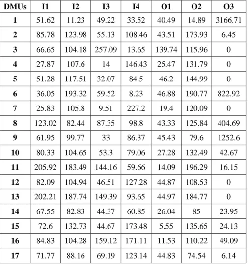
To illustrate the merits of the proposed approach, we choose an example from Kao and Hung (2005). In that example, 17 forest districts (DMUs); four inputs (I1-I4): budget (in US dollars), initial stocking (in cubic meters), labor (in number of employees), and land (in hectares); and three outputs (O1-O3): main product (in cubic meters), soil conservation (in cubic meters), and recreation (in number of visits) are considered for measuring the efficiency.

Table 1 contains the original data, while Table 2 shows the common set of weights generated by the proposed method (GP), with respect to inputs and outputs. Furthermore, Table 3 shows the efficiency scores of the 17 forest districts calculated from the CCR Model, efficiency scores of the compromise solution approach by Kao and Hung (2005), and the efficiency scores of the GP approach in this paper, respectively.

Table 1. Input and output data for the 17 forest districts in Taiwan.

DMUs I1 I2 I3 I4 O1 O2 O3

1 51.62 11.23 49.22 33.52 40.49 14.89 3166.71

2 85.78 123.98 55.13 108.46 43.51 173.93 6.45

3 66.65 104.18 257.09 13.65 139.74 115.96 0

4 27.87 107.6 14 146.43 25.47 131.79 0

5 51.28 117.51 32.07 84.5 46.2 144.99 0

6 36.05 193.32 59.52 8.23 46.88 190.77 822.92

7 25.83 105.8 9.51 227.2 19.4 120.09 0

8 123.02 82.44 87.35 98.8 43.33 125.84 404.69

9 61.95 99.77 33 86.37 45.43 79.6 1252.6

10 80.33 104.65 53.3 79.06 27.28 132.49 42.67

11 205.92 183.49 144.16 59.66 14.09 196.29 16.15

12 82.09 104.94 46.51 127.28 44.87 108.53 0

13 202.21 187.74 149.39 93.65 44.97 184.77 0

14 67.55 82.83 44.37 60.85 26.04 85 23.95

15 72.6 132.73 44.67 173.48 5.55 135.65 24.13

16 84.83 104.28 159.12 171.11 11.53 110.22 49.09

17 71.77 88.16 69.19 123.14 44.83 74.54 6.14

Table 2. A common set of weights generated from GP method.

v1 v2 v3 v4 u1 u2 u3

0.20026 0.34628 0.00010 0.03421 0.06658 0.35022 0.00236

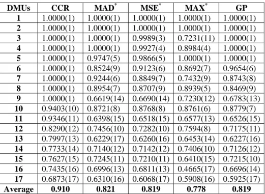
The CCR efficiency scores are the highest values that the districts can attain, and there are nine efficient units which cannot be differentiated. Regarding the compromise solution approach (Kao and Hung, 2005) three values of p, viz., 1, 2, and

∞

, have been considered and the results are referred to as MAD, MSE and MAX.

The common sets of weights generated from these four models, on whose basis the efficiency scores of every district are calculated, are different sets of weights due to the fact that they are obtained from different viewpoints. Therefore, it is inappropriate to say which weights are correct and which are not. But, as Kao and Hung (2005) mention, the property that the distance between the vector of efficiency scores calculated from the compromise solution approach to the efficiency scores calculated from the standard DEA model, is the shortest in the Euclidean space, suggests that

p=2 is the most suitable choice in compromise solution approach. Therefore, to be conservative,

correlation coefficient). Like the Pearson product moment correlation coefficient, Spearman’s ρ is a measure of the relationship between two variables. However, Spearman’s ρ is calculated on ranked data.

Table 3. Efficiency scores and the associated rankings (in parentheses) calculated from the CCR ratio model for different methods of common weights.

*Results obtained from Kao and Hung (2005).

DMUs CCR MAD* MSE* MAX* GP

1 1.0000(1) 1.0000(1) 1.0000(1) 1.0000(1) 1.0000(1)

2 1.0000(1) 1.0000(1) 1.0000(1) 1.0000(1) 1.0000(1)

3 1.0000(1) 1.0000(1) 0.9989(3) 0.7231(11) 1.0000(1)

4 1.0000(1) 1.0000(1) 0.9927(4) 0.8984(4) 1.0000(1)

5 1.0000(1) 0.9747(5) 0.9866(5) 1.0000(1) 1.0000(1)

6 1.0000(1) 0.8524(9) 0.9123(6) 0.8692(7) 0.9654(6)

7 1.0000(1) 0.9244(6) 0.8849(7) 0.7432(9) 0.8743(8)

8 1.0000(1) 0.8954(7) 0.8707(9) 0.8939(5) 0.8469(9)

9 1.0000(1) 0.6619(14) 0.6690(14) 0.7230(12) 0.6783(13)

10 0.9403(10) 0.8721(8) 0.8768(8) 0.8761(6) 0.8779(7)

11 0.9346(11) 0.6398(15) 0.6518(15) 0.6577(13) 0.6526(15)

12 0.8290(12) 0.7456(10) 0.7282(10) 0.7594(8) 0.7175(11)

13 0.7997(13) 0.6229(17) 0.6260(16) 0.6453(14) 0.6227(16)

14 0.7733(14) 0.7140(12) 0.7142(12) 0.7406(10) 0.7126(12)

15 0.7627(15) 0.7245(11) 0.7210(11) 0.6410(15) 0.7215(10)

16 0.7435(16) 0.6996(13) 0.6811(13) 0.4665(17) 0.6696(14)

17 0.6873(17) 0.6310(16) 0.6068(17) 0.5908(16) 0.5925(17)

Average 0.910 0.821 0.819 0.778 0.819

For calculating spearman’s

ρ

we can use the following formulation in which

_d

_i is the difference between ranks for the same observation (DMU) and n is the number of DMUs.

)

1

(

1

2 1

2

−

−

=

∑

=

n

d

r

n

n i i s

As an alternative, we can compute the Pearson’s correlation on the columns of ranked data. The result of this formulation is too close to the exact Spearman’s

ρ

. In this formulation

x

i

,

y

iare the ranks for the same DMUi. And i=1,2,3,…,n.

2 1

2 2

1 2 1

.

n

y

x

n

y

x

n

r

n

i i

n i i

n i i i

y

x

y

x

−

−

−

=

∑

∑

∑

= =

=

Empirically, in this example the spearman’s correlation between the set of efficiency scores of the GP method and MSE (where p=2), is greater than 95%. However, GP approach needs to solve a linear problem and this is its advantage of it over the Kao and Hung’s approach, which has to solve a nonlinear problem. In general, the rankings of these four methods, as shown in parentheses in

Table 3, are consistent with those of the CCR model, indicating that the results are reasonable. In addition, they are more informative. Not only do they differentiate the efficient units, but also detect some abnormal efficiency scores calculated from the CCR model. The efficiency scores obtained for districts 9 and 11 are two of such examples.

5. CONCLUSIONS

The flexibility in the choice of weights is both a weakness and a matter of strength for DEA approach. It is a weakness because it tends to deter the comparison among DMUs on a common basis. This flexibility is also a sign of strength, however, for if a unit turns out to be inefficient even when the most favorable weights have been incorporated in its efficiency measure, then this is a strong statement and in particular the argument that, the weights are incorrect is not tunable.

For dealing with this difficulty and assessing all the DMUs on the same scale, this paper proposes the application of goal programming approach for generating common set of weights. There are other methods in the literature which are also able to generate common weights. A case taken from Kao and Hung (2005) is solved to investigate the differences among these methods and some conclusions are derived.

Solving linear problems is an advantage of the proposed approach against general approaches in the literature which are based on solving nonlinear problems. When weights of the input/output factors are available, efficiency scores can be measured. Moreover, all DMU’s can be ranked in terms of a common basis. Compared to the original DEA model, this approach discriminates in a better way among DMU’s in order to yield the less efficient ones. As in the conventional DEA model, it does not require the formulation of n models. In fact, the efficiencies of all DMU’s can be calculated by solving a single model, enabling one to evaluate the relative efficiency of every DMU on a common weight basis. Finally, with appropriate modifications, the proposed method, can simply be generalized to other DEA models.

REFERENCES

[1] Bouyssou D. (1999), Using DEA as a tool for MCDM: some remarks; Journal of the Operational Research Society 50(9); 974-978.

[2] Charnes A., Cooper W.W. (1961), Management Models and Industrial Applications of Linear Programming; John Wiley, New York.

[3] Charnes A., Cooper W.W., Rhodes E. (1978), Measuring the efficiency of decision making units; European Journal of Operational Research 2; 429-444.

[4] Doyle J.R., Green R.H. (1994), Efficiency and cross-efficiency in DEA: derivatives, meanings and uses; Journal of the Operational Research Society 45; 567-578.

[5] Estellita Lins M.P., Angulo Meza L., Moreira da Silva A.C. (2004), A multi-objective approach to determine alternative targets in data envelopment analysis; Journal of the Operational Research Society 55; 1090-1101.

[6] Giokas D. (1997), The use of goal programming and data envelopment analysis for estimating efficient marginal costs of outputs; Journal of the Operational Research Society 48(3); 319-323.

[7] Golany B. (1988), An interactive MOLP procedure for the extension of DEA to effectiveness analysis; Journal of the Operational Research Society 39(8); 725-734.

[8] Golany B., Yu G. (1995), A goal programming-discriminant function approach to the estimation of an empirical production function based on DEA results; Journal of Productivity Analysis 6; 171-186. [9] Jahanshahloo G.R., Memariani A., Lotfi F.H., Rezai H.Z. (2005), A note on some of DEA models and

finding efficiency and complete ranking using common set of weights; Applied Mathematics and Computation 166; 265-281.

[10] Joro T., Korhonen P., Wallenius J. (1998), Structural comparison of data envelopment analysis and multiple objective linear programming; Management Science 44; 962-970.

[11] Kao C., Hung H.T. (2005), Data envelopment analysis with common weights: the compromise solution approach; Journal of the Operational Research Society 56; 1196-1203.

[12] Karsak E.E., Ahiska S.S. (2005), Practical common weight multi-criteria decision-making approach with an improved discriminating power for technology selection; International Journal of Production Research 43(8); 1537-1554.

[13] Kornbluth J. (1991), Analysing policy effectiveness using cone restricted data envelopment analysis; Journal of the Operational Research Society 42; 1097-1104.

[14] Roll Y., Cook W.D., Golany B. (1991), Controlling factor weights in data envelopment analysis; IIE Transactions 23(1); 2-9.

[15] Roll Y., Golany B. (1993), Alternate methods of treating factor weights in DEA; Omega 21(1); 99-109.

[16] Stewart T.J. (1996), Relationships between data envelopment analysis and multicriteria decision-analysis; Journal of the Operational Research Society 47(5); 654-665.

[17] Xiao Bai L., Reeves G.R. (1999), A multiple criteria approach to data envelopment analysis; European Journal of Operational Research 115; 507-517