UNC_Bachelor_Thesis_in_Mathematics.pdf

(1)

Assessing the Scalability of Parallel

Programs: Case Studies from IBAMR

Elijah DeLee

SENIOR HONORS THESIS

Mathematics Department

University of North Carolina at Chapel Hill April 2018

Approved:

Boyce Griffith, Ph.D. Thesis Advisor

Katie Newhall, Ph.D Reader

(2)

(3)

I declare that I carried out this bachelor thesis independently, and only with the cited sources, literature and other professional sources.

(4)

Abstract

Title: Assessing the Scalability of Parallel Programs: Case Studies from IBAMR

Author: Elijah DeLee

Supervisor of the bachelor thesis: Boyce Griffith, Ph.D.

Abstract:

Programmers are driven to parallelize their programs because of both hardware limitations and the need for their applications to provide information within ac-ceptable timescales. The modelling of yesterday’s weather, while still of use, is of much less use than tomorrow’s. Given this motivation, those researchers who build libraries for use in parallel codes must assess the performance when deployed at scale to ensure their end users can take full advantage of the computational resources available to them. Blindly measuring the execution time of applications provides little insight into what, if any, challenges the code faces to achieve op-timal performance, and fails to provide enough information to confirm any gains made by attempts to optimize the code. This leads to the desire to gain greater insight by inspecting the call stack and communication patterns. The author reviews the definitions of the forms of scalability that are desirable for different applications, discusses tools for collecting performance data at varying levels of granularity, and describes methods for analyzing this data in the context of case studies performed with applications using the IBAMR library.

(5)

Chapter 1 Introduction

Programmers are often driven to parallelize programs by two different desires, either they want the results from a program with a fixed workload faster, or they want to solve a larger problem in the same amount of time as it took to solve a smaller problem. Whether the parallelization of a program isscalableis a metric of how successful the implementation is at achieving these ends. These end goals are disparate enough that they deserve two different metrics for measuring how successful we have been at achieving them.

First, I will review the definitions of these types of scalability. Then I will discuss what barriers programmers face in both ascertaining and achieving scal-ablity. Finally, I will discuss what we hope to get out of any assessment of the scalability of a program. This information will frame the method in which cases studies were performed and the results found.

1.1 Defining scalablity

If a program must perform many computations on a limited data set, this is generally termed compute bound. It may make sense to say that we would like to devote more hardware to the problem and expect a solution in a shorter amount of time. If we rework this program to split the computational steps over more processors, when we evaluate whether or not we have achieved our goal, we should be concerned with strong scalibility. More formally, a program exhibits strong scalability when its time to solution decreases in proportion to the increase in processors given a fixed “problem size”. A classic compute bound problem is brute force encryption cracking. If we are in the business of de-encrypting data we do not have the private key to, then our workload is fixed, and we are interested in using more hardware to arrive at a solution faster.

Because we cannot expect perfect strong scalability, it is common to define two terms to help us asses how strongly scalable a program is. If the time a program takes to execute in serial is Tserial and the time it takes to execute in

parallel is Tparallel, speedup, S, is defined as:

S = Tserial

Tparallel

(7)

run of the program):

E = S

nprocessors

= Tserial

nprocessorsTparallel

Unlike a compute bound problem, a memory bound problem faces limita-tions to its run time not because of the time it takes for computalimita-tions to complete on the processor, but because it takes time to load the data into memory. Most modern computers have been built exploit a hierarchy of memory, keeping re-cently used data in very “fast” memory in the form of the processor’s registers and cache, the rest residing in much slower main memory, and when this fails to hold the data it may also be written to disk (“swap”), which is extremely slow. Beyond the question of the speed of memory, there are physical limitations to how much memory can be on a chip (cache size), and to the volume of memory that can be transferred to the chip in any given amount of time (memory bandwidth). These factors support a upper bound to any gains in efficiency optimization of data access patterns can hope to achieve. So when a programmer parallelizes this type of code, it is with the hope that spreading the data over more nodes can effectuate a improvement in the execution time because each node has less data to work through and can fit a greater proportion of the data in faster memory. Also, it is quite possibly the case that the program simply has memory needs that exceed the memory available on any single machine that the user has access to. In this case, if the problem can be partitioned into smaller problems and spread out over several machines, then it transitions from being “completely unsolvable”, to “solvable”, which provides an excellent speedup factor of an immeasurable quantity. In cases such as this, there is no sensible way to compare the parallel program with the serial version, because it may simply be impossible to run our program in serial on any hardware we have access to.

In the case of memory bound applications there is likely an ideal ratio of “work” to each “worker”. We can quantify “work” as the volume of data, since this is our limiting factor, and the “workers” as CPU cores, as this is how we will distribute the work. If we can find this ideal proportion1_{, and keep this ratio of}

data to number of CPU cores constant, we would hope to be able to solve a larger problem in the same amount of time as it took us to solve a smaller problem. This is what is called weak scalability, when the time to solution stays constant as we increase the amount of computational resources in proportion to the growth in problem size.

Many numerical schemes for basic matrix operations provide the classic exam-ple of memory bound algorithms. Often matrices and arrays are used to represent data on a spatial grid, such as in the fluid structure interaction problems users of IBAMR implement. In this use case, if we want to run our simulation with a certain resolution of the spatial grid, we would hope to be able to run the program at a low resolution on a set number of nodes in an acceptable amount of time, and then and then scale the number of nodes in proportion to the resolution of the grid and still get our solution in roughly the same amount of time.

1_{Performing trials to determine this ideal problem size to compute power ratio is referred to}

(8)

1.2 Challenges to scalability

Parallelizing programs must come at some cost, at least because of the cost of communication unless a problem is of the class of “embarrassingly parallel” problems2_{. The communication itself is limited by the rate and volume at which}

data can be transmitted from one process to another. Additional costs are also incurred by the software that makes this communication possible.

1.2.1 MPI Communication Overhead

IBAMR and several libraries it depends on, including PETSc, [2], and SAM-RAI, [3] utilize the MPI standard3 to enable their programs to be run on dis-tributed memory systems, where separate processes (also referred to as “ranks”) each only have direct access to their own memory address space, and perform other communication and data access over the network.

Network latency and bandwidth then contribute to the time to solution, an-nulling some of the gains that the parallelization may have achieved. Much research is devoted to the limitations provided by network communication and the network topology of high performance computing clusters. In general, the programmer would like to be agnostic of these details and write a program that runs well on any system that provides the necessary runtime environment. But it is important to note the fact that performance can vary greatly from one clus-ter to another, and even from one run on a clusclus-ter to another depending on the distribution of the nodes in the network provisioned by the cluster’s scheduling system.

Because network communication is expensive, it is important to design our al-gorithms to divide the workload as “evenly” as possible, as whenever one node is waiting, it means that another is working harder than it needs to be. IBAMR uses adaptive mesh refinement (AMR), to discretize different portions of the compu-tational domain at different levels of refinement. This process occurs throughout simulations, causing a great variability in total workload. The domain is di-vided into “patches” that are then distributed to the ranks. These patches are redistributed as some interval, and this is a step that is fraught with possible performance issues if data locality is not properly considered by the distribution algorithm.

Using MPI also incurs other incidental costs that may not be obvious to those who have only considered parallel computing from a distance. Initializing the MPI communication infrastructure takes a non-trivial amount of time that increases at a rate that is at least O(n), if not O(n2), n being the number of nodes or CPU cores. The cost of this set up stage can be amortized over longer running programs, but it can dominate the execution time if the workload of the program is too small. A programmer attempting to assess the scalability of their code should to take this into consideration when designing their profiling trials.

2_{Embarrassingly parallel problems are those where no communication between each parallel}

process is necessary because each process acts on data that is not effected by the results of the other processes.

3_{The MPI standard (Message Passing Interface) is implemented by various libraries,}

(9)

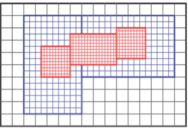
Figure 1.1: Graphical depiction of a mesh with various patches of different levels of refinement.The patches, outlined in bold, are distributed to the ranks. So-called “ghost cells” exist on the boundaries of each patch to allow each patch access to the cells that are directly adjacent to it. The process of filling these ghost cells requires communication between the ranks. Source: Presentation by Ann S. Almgren, Lawrence Berkeley National Laboratory [6]

The MPI implementation may also do other work that can have unexpected consequences. One such activity is so called “busy waiting”. Both MPICH and OpenMPI use “busy waiting”. In summary, it is common to use “helper” threads spawned by each rank to check to see if anything needs to be done (for example, receive data that the rank has been sent). These helper threads can be very active and if more processes have been spawned than there are available cores, the helper threads will end up interrupting the execution of the actual program. This can have horribly detrimental effects on the performance of the program and can lead to very misleading results when analyzing scalability. This provides another constraint when designing what weak scaling trials should look like.

1.3 Problem size

As mentioned before, IBAMR’s fluid solvers utilize algorithms that are con-sidered classically memory bound. Generally the computational domain is fixed to a certain region of interest, but the level of refinement of the spatial grid is configured by the user at runtime in an input file. Because of the nature of pro-grams that use adaptive mesh refinement, memory usage of the program evolves over time. The most defining factors of how much memory will be consumed are the initial grid spacing, the ratio at which the grid is refined at each level of refinement (notice the finer grid spacing of the smaller patches in figure 1.1), and the number of levels of refinement allowed4.

As will be discussed at further length, the goal of the scaling study should be a guiding principle when it comes to defining what the problem size is. If the goal is primarily to provide results that guide refactoring of code to produce measurable

4_{These parameters are referred to in IBAMR input files as follows: The initial discretization}

(10)

benefits to the scalablity of the program that are meaningful to the end user and utilize computational resources in a cost effective manner, the problem size should be defined in the simplest possible manner that garners these results. Given this guidance, the problem size will be considered the number of cells in the initial level of refinement. For example, in a three dimensional simulation, if the initial number of cells on one face of the cubic domain is 64, then the initial number of cells is 643 _{= 262144. For simplicity I will often refer to simply the refinement}

of one face, which in this example is 64. Other measures of “problem size”, for example the number of time steps in a simulation that models the evolution of the fluid on the spatial grid over time, will be fixed to isolate the resolution of the spatial grid as the only parameter measuring workload in the study.

1.4 Formative Assessment of Performance

Despite the fact that it is unlikely to achieve perfect scalability, it is very likely that we can improve the scalability of a program. Attempting to guess where the inefficiencies in a program are is likely to result in what is colloquially termed “Premature Optimization”. Moreover, even if we blindly refactor code in an attempt to improve its efficiency, it is difficult to accurately gauge to results of our optimization if we simply measure time to solution. We may very well have improved one portion of our program but incurred some kind of incidental loss of performance in another region of the code. Another consideration specific to the types of simulations built with IBAMR is the fact that we are quantifying “problem size” on the refinement of the spatial grid, but the computation models the fluid-structure interaction as it evolves over time. In this case, there may be costs incurred in initializing MPI or setting up the solver that are one time costs. This means that these portions of the program have diminishing relative cost when the simulation is run for more time steps. This means we are not equally concerned with the scalability of all portions of the code, because they have varying impacts on time to solution. It would provide much clearer gains to the end user for the solve step to be scalable rather than the initialization of the solver, because many solve steps are performed in a simulation, but the solver is only initialized once.

(11)

Chapter 2 Methods

This section will describe the tools used to asses the scalability in each of the case studies as well as the formulation of the case studies and the configuration of the tools for each study.

2.0.1 Methods to gain introspection

There are a handful of data sources that most profiling tool-chains use to gain introspection into the program flow across the many processes of a par-allel program. I have concerned myself exclusively with the tools available for C/C++/FORTRAN based programs.

There are two primary avenues for collecting the data. The first is to in-terrupt the program at some configured rate and make observations. This is accomplished by running the parallel process through another process, which fa-cilitates monitoring when libraries are loaded and unloaded. In this case it is not necessary to insert any additional code into the original program to gain insight into what functions are running at any given time. This produces a statistical view of the runtime, telling you what percentage of the time the monitoring pro-cess found itself in each portion of the code. In this method, the amount of overhead the measurement generates is proportional to the sampling frequency, not the frequency of calls or depth of the call stack. Inevitably, because the tool is interrupting the program flow on the chip and performing some amount of action itself, it can perturb the counts on the very hardware counters that it is using to assess the program. The programmer can choose to accept this perturbation as small enough if the sampling frequency is low enough to not be statistically significant.

Alternatively, some tools instrument code by inserting statements into code to generate metrics, producing data about how long a function executed for by collecting the time at entry and the time at exit. The instrumented code is executed as normal, and the metrics are generated at runtime. The process of instrumentation may be manual or automated. Instrumented code generally will execute slower from the user’s perspective compared to the previous method, but does not perturb the measurement of the time for sections of the code that it is measuring. The cost of a slower executing program may be non-trivial depending on the computational resources available to the programmer.

(12)

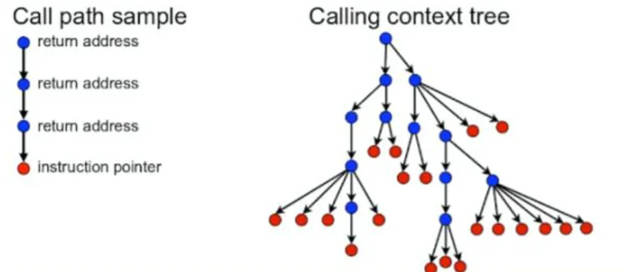
Figure 2.1: Graphical depiction a calling context tree reconstructed by inspecting the call stack at the time of measurement and using the return address to identify the caller. Adapted from hpctoolkit.org: [9]

methods have their implicit costs.

A commonality between the methods is that they generally leverage two C libraries libunwind [7] and PAPI [8]. The libunwind library facilitates intro-spection into the call chain of a program. This can be used to display the data in a calling context tree, and to calculate metrics such as the “exclusive” execution time of a function call (eg, subtracting the time or other metric that child items are responsible for from the parent item.) The PAPI library provides a consistent interface to hardware counters many performance analysis tools use in an effort to be platform independent. This is necessary because chips from different man-ufacturers often has different APIs for the hardware counters that collect data, for example the number of FLOPs computed in a certain number of cycles. Both are freely available as source code to be built by the user.

These tools can then be used to assess how much time each rank spend in each function call, or other metrics including how many floating point operations were performed in a function call.

In the case studies performed, I used tools from both types and will comment on the user experience of both in further detail in the discussion section.

2.0.2 Presentation and Analysis of the data

These data are then generally presented in two modes, called profiles and event traces. In a profile, the time dimension is compressed, giving a sum of a metric over the course of the program and associating it with items in either a calling context tree, giving us a sum for each node in the tree over the course of the program, or a flat view where all instances of a function call are squashed as well, giving us a sum over the course of the entire program. In the flat view, each function call is shown with its sum total of the metric in question, as it may be the child item of several higher level functions. A calling context tree (as shown in 2.1), displays the metric associated with each function call as a node in a tree, as shown in figure 2.2. If an function call f1 is called by both f2 and f3, it will appear as a child item of both in the tree.

(13)

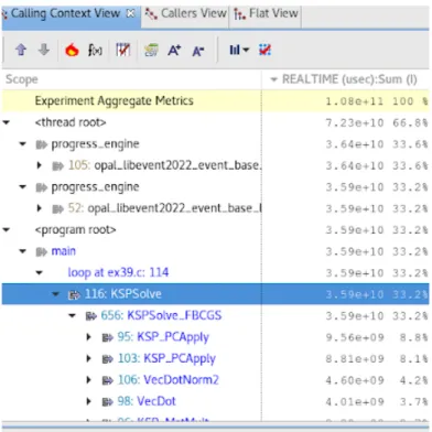
Figure 2.2: In a profile, the time dimension is compressed and we are presented with a single metric for each item in the call tree.

must be done with care, as some times it may appear that one function is to blame when it is not in reality the bad actor. This is because there a function may have a barrier at the end, but have no blocking wait before the function call. So it may appear that the program spent a large deal of time in a function, but in actuality the load imbalance lays in the function call before it. This scenario is illustrated in figure 2.3.

For this reason, a second mode of presentation is often used called a trace view. To generate the trace view, much more data must be collected than is needed to generate the profile view. The trace view generates what can be conceived of as a three dimensional view of the program’s execution. Generally, we are presented with colorized data where each function call is assigned a color, and we can see in each process at each unit of time what function call the program

(14)

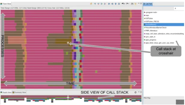
Figure 2.4: This labeled screenshot of HPCToolkit’s trace viewer (aptly named

hpctraceviewer) shows all elements expected in a trace visualization. These are: a plot with each process colorized to indicate what function it was found in at each measured time slice at one layer of the call stack, a side view of all the layers of the call stack, and a legend relating the colors to function calls.

was in. This data is layered, so at each instance of time in each process we can navigate through the layers of the call stack. These attributes are illustrated in figures 2.4 and 2.5.

2.1 Tool Selection

Various additional factors placed constraints on the choice of tool selection. These include the cost, if any, to acquire any of the tools or data presentation software, the compatibility of any of the tools with the platform that the pro-grammer has available to them, and personal preference when it comes to the user experience of any of the profiling software.

(15)

Figure 2.5: Conceptual drawing of the trace view from HPCToolkit presentation by John Mellor-Crummey [10]

chains. All of the HPCToolkit tools are free, and the profiling portion of the Score-P ecosystem is also free. It is the case that the Score-P trace generation tool is free, and the file format of the traces is open source, but there are no currently active projects (at the time of writing) other than the non-free Vampir [13] trace viewer to consume this trace data.

Returning again to the primary motivation of this study, which is to derive actionable information about the scalability of different portions of IBAMR, I would have been well served to be even more prejudiced about the difficulties I might face as a user of the profiling tools. Challenges faced building and run-ning, storing and moving the data generated, as well as viewing and otherwise consuming the data generated, all slow the process and take available time away from achieving the primary goal, which is assessment and improvement of the scalablity of the software under study. That said, once you have chosen a tool, there is a certain amount of investment made that is difficult to justify throw-ing away at the first roadblock. This includes time readthrow-ing documentation as well as building the environment that the tool requires. It is common knowledge among users of scientific software that navigating a myriad of user configured and built C/C++/Fortran libraries can “inhibit software evolution by imposing an unintentionally-high cost to change and dilution of effort to meet short-term deliverables, ” [14].

2.2 Preparing the weak scaling trials

Two case studies were performed, each with one of the tool chains named above, HPCToolkit and Score-P. I will describe any special preparation of the application for profiling as well as the design of the scaling trials.

(16)

So while they are working independently and are not being actually interrupted by each other, they still are in effect “waiting in line” for memory. For this reason we fixed the number of cores at 8 per node, well below the total 22 cores on each node.

To attempt to control for user error, which there were ample opportunities for, I created templates for the submission script and input files for the application, to ensure each trial was doing the exact same simulation and only varying the grid spacing and the number of nodes on which it was running. Additionally I disabled all visualization data output, as this time consuming activity of writing to disk would obscure the phenomena I was attempting to observe, which is the performance of the solver. Additionally I logged information regarding the the grid spacing and the number of cores the run was using in the logging of stdout

and stderr that the scheduling system provides jobs. Finally, I separated the data by creating a directory structure such that each trial would output its logs and profiling data into directories whose names encoded information about the run.

Additionally, I had the submission scripts create symbolic links to the same binary of the application, so as to ensure that all trials were running the same compiled program and only varying the input file.

experiment root folder

nodes 1

N 128 submit.sh

nodes 2

N 160 submit.sh

Diagram of directory structure of a weak scaling trial.

2.2.1 Case Study 1: Linear Solver with HPCToolkit

The only specific compile-time requirement for preparing the application for profiling with HPCToolkit’s hpcrun is to compile the IBAMR library and all dependencies with the -g compiler flag that tells the compiler to include extra debugging data when producing the symbols, which allows hpcrun to link the symbols it encounters back to the original source code.

(17)

is generally used in the types of simulations users build with IBAMR where the solver is used many times as the simulation evolves over time.

Initially, I was attached to the idea that I would double the refinement of the coarsest level of mesh and increase the number of cpus by a factor of 8 for each run in the weak scaling trial. This yielded two issues, the first being only 4 possible runs were possible on the cluster I was interested in, that being with 1 node, 8 nodes, 16 nodes, and 128 nodes. The second problem was that submitting a job to use 128 nodes of a cluster that has only 183 nodes yielded unacceptable wait times for it to progress through the queue (a week or more). This motivated me to consider intermediate multiples of the initial workload, to give me data points that were less dispersed. I finally decided on scaling the grid spacing by 11₄ with each run. This resulted in the configuration displayed in the following figure.

Second Design for Weak Scaling Trials (3D domain)

N Cells Nodes Cores Cells/Core

128 2097152 1 8 262144

160 4096000 2 16 256000

200 8000000 4 32 250000

250 15625000 8 64 244140.63

316 31554496 16 128 23478.05

391 59776471 32 256 233501.84

More details arose in discussion with other IBAMR developers that informed my design of the trials for this second program.

It is a commonly held belief among IBAMR developers that the algorithms IBAMR and SAMRAI use can display poor performance or odd load balance when the number of grid cells can not be evenly divided by the number of MPI ranks. This is by the basic nature that patches are distributed to each rank and each rank gets at least one patch, and patches must consist of integer numbers of cells.

Because of the additional constraint of desiring the base grid spacing to be evenly divided by the number of cores, I decided it was acceptable to perturb this value a small amount to arrive at a convenient number whose cube was divisible by the number of cores. This resulted in the configuration displayed in the following figure.

Final Design for Weak Scaling Trials (3D domain)

64 262144 1 8 32768

80 512000 2 16 32000

100 1000000 4 32 31250

128 2097152 8 64 32768

160 4096000 16 128 32000

200 8000000 32 256 31250

(18)

[16]. HPCToolkit generates profiles that are relatively large because they include a copy of the entire source code tree that it finds when doing the static analysis of the binary.

Collecting the trace data with HPCtoolit generates data files on the order of gigabytes. This is much larger than the data files generated when only collecting profile data with HPCToolkit, which is on the order of megabytes. I could not find any practical way to compare the trace data across runs. For these two reasons, I only collected the trace data for the largest run as a means to look to see if load imbalance was a problem.

2.2.2 Case Study 2: 3D ABC Flow with Score-P

The second case study used the Score-P tools to collect data from running a three dimensional periodic flow simulation of a classical problem that has an analytic solution, used by IBAMR developers as a model problem for convergence study of the solvers. The simulation is of what is termed the “Arnold-Beltrami-Childress” flow1 with periodic boundary conditions [17]. The general form is given by equation 2.1.

uA,B,C(x, y, z) = (Asinz+Ccosy, Bsinx+Acosz, Csiny+Bcosx) (2.1)

This simulation uses refinement but does not use AMR, in that the levels of refinement do not change size or location in the domain.

Building Score-P with my initial choice of compilers, OpenMPI using gcc 4.8, on the cluster I was working on was uneventful and mislead me to think that this would be the case were I to build it on another system or with another set of compilers. This proved not to be the case upon further investigation, but was not an issue for the completion of this case study, seeing as it worked “out of the box” in this scenario.

To profile an application with Score-P it is necessary first build Score-P with the compiler of choice, and then to compile the application with the Score-P wrapped compilers and any libraries that the application depends on to the extent of the interest of the researcher doing the profiling. I started with only compiling IBAMR and the application with the Score-P wrapped compilers.

Score-P provides some ability to narrow the regions of the code where profile and trace data is collected. This helps to greatly reduce the size of the profile as well as make the data easier to consume for the end user, yielding much less cruft and flotsam to sort through in the search for the part of the code you are interested in. The filtering can be informed by running an small test of your program and analyzing the resultant profile with a tool that is built along side the other Score-P tools called scorep-score. This tool provides metrics about how large the trace would be and what calls are responsible for the size of the profile.

This data may be helpful to some, but did not provide any information I was able interpret, other than the profile would be very large if I did not do anything to trim it down. A direct way narrow the focus of the profile that I chose was to

(19)

define my own custom “region” name and create a filter file that instructs Score-P to ignore everything outside of that region. By wrapping the solve step with the a macro provided by including a header from the Score-P source code, I was able to reduce the size of the profile down to a size where I could compress the whole directory tree for the entire set of weak scaling trials down to an archive less than 100 megabytes in size. All child items of this root call are included in the profile.

#include <scorep/SCOREP_User.h>

// ... omitting unrelated code ...

SCOREP_USER_REGION_DEFINE(solve)

SCOREP_USER_REGION_BEGIN(solve, "solve", SCOREP_USER_REGION_TYPE_FUNCTION)

// main solve step

time_integrator->advanceHierarchy(dt) SCOREP_USER_REGION_END(solve)

// ... omitting unrelated code ...

The documentation about the arguments to these macros consists of an exam-ple in the user manual, with out any explicit acknowledgement of what becomes of these arguments. Given this lack of guidance, I chose to keep things simple and give it all the same name.

After creating this named region in the source code, I then was able to cut the profile down to a very reasonable size by creating the following “filter file” and alerting Score-P to its presence by exporting its path to an environment variable2

in my submission script.

SCOREP_REGION_NAMES_BEGIN EXCLUDE *

INCLUDE *solve* *SOLVE*

*advanceHierarchy* *Hierarchy*

SCOREP_REGION_NAMES_END

The method by which the string matching worked, which allows for wildcards like “*”, was not clear from my reading of the documentation. Primarily, it is unclear if the string matches act on the mangled names or on the unmangled names. For this reason I erred on the side of being over zealous. The goal was to cut down on the amount of noise and the size of the profile while not excluding information I needed, which this filter achieved. If it still captured information I did not end up needing, that was not of importance to me. The guiding principle of “what will provide me with information that I can act on to improve my program” again informed me to not spend much time optimizing this filtration process.

(20)

If Score-P encounters a function call that calls into another library, its child items may not be present in the profile data if these functions do not have pub-lic symbols defined. This was the case in a function that I was interested in investigating further upon initial trials that resided in SAMRAI. To make this information visible in the profile, I again created a custom user region in the source code for the function I was interested in and rebuilt SAMRAI with the Score-P compilers. This made the private SAMRAI function’s data appear as a child item of the public SAMRAI call that had piqued my interest because of its behavior (which will be discussed at more length in the results section).

While the compiler emitted warnings about multiple definitions of some Score-P macros because of the fact that the header was included in the SAMRAI library as well as the IBAMR application, everything appeared to function normally.

Having added this region, named “overlapping box” in homage to the function name, I added it in various permutations to my Score-P filter file, including the name of the function itself.

SCOREP_REGION_NAMES_BEGIN EXCLUDE *

INCLUDE *solve* *SOLVE*

*advanceHierarchy* *Hierarchy*

*makeNonOverlappingBoxLists* *overlapping_box*

*overlapping* SCOREP_REGION_NAMES_END

The final configuration of grid spacing to number of processors used for the Krylov sovler was used again for this study.

Weak Scaling Trials for ABC Flow Simulation (3D domain)

64 262144 1 8 32768

80 512000 2 16 32000

100 1000000 4 32 31250

128 2097152 8 64 32768

160 4096000 16 128 32000

200 8000000 32 256 31250

2.3 Data Analysis

2.3.1 HPCToolkit Data

After collecting the profile data during the run of the program with hpcrun, it is necessary to merge the data with the output of the static analysis tool

(21)

unreliable. They would intermittently fail to be able to merge the data, appearing to have issues related to excessive recursion causing the Java Virtual Machine to run out of memory. I was able to avoid trouble shooting this problematic behavior by switching to the other version whenever the one I was using was not working. So if hpcprof-mpi broke on the merge step, I would switch to hpcprof. This workflow did not engender in me a great trust of the tool kit.

There are various command line options to generate different statistics from the event data. I chose to use a catch all that would produce the average, sum, standard deviation, inclusive and exclusive time metrics.

The workflow for each trial then looked (roughly) like this:

# Perform static analysis, creating main3d.hpcstruct > hpcstruct main3d.cpp

# Run the program, generating measurements directory > hpcrun --event REALTIME@6000 ./main3d input3d # Merge the static and runtime data

> hpcprof -S main3d.hpcstruct -I./’*’ hpctoolkit-main3d-measurements -M stats # archive results to transport to workstation to use GUI data viewer

> tar -cjf database.tar.bz2 *database*

This database is consumable by the hpcviewer tool, which has a graphical interface. The data viewer is available in pre-compiled binary format for download on the HPCToolkit website.

I would then bring these files down to my local workstation via scp because other methods of connecting remotely to the database proved to have too much latency for me to be able to do any meaningful work.

At this point in the project I was still guilty of some “premature optimization” of my workflow, attempting to perform my data analysis and graph generation with scripts. Initially I attempted to work with another of the HPCToolkit util-ities,hpcdata [18], a command line tool that can consume the data format pro-duced byhpcprof. This did not prove fruitful. The second workflow I attempted to use was as follows:

1. Download archive of merged database and unpack

2. Open the database with hpcviewer

3. Export the data to csv with a button

4. Load the csv data into a python object provided by thepandas library

For the first trials I went through several more stages mangling this csv data in python scripts to attempt to “automate” the generation of various figures. This proved time consuming, spending a good deal of time dealing with various inconsistencies in the string formatting of the data.

(22)

More specifically, if the function name is in columnA of a spreadsheet, and data from the 2 node case is in a sheet named nodes2, the spreadsheet software I used (Google Sheets) allowed me to search through the nodes2 sheet and copy a certain cell in a row if the corresponding columnA cell had the same value as my reference sheet with an equation called VLOOKUP. Documentation on the VLOOKUP function can be found on the Google Docs help pages [19].

2.3.2 Score-P Data

My endeavor to automate the data analysis of the HPCToolkit data had sufficiently humbled me by the time I approached the profile data of Score-P. Given this experience, I chose to not investigate how to script the extraction of the data from the profile data. Instead I chose a very simple method that provided me intelligible insight into the results with little over head.

The data viewer for the profile data,cube, was available via my workstation’s operating system’s package manager (Fedora 25, usingdnf). This worked without any customization. I then performed the following steps to generate graphs that compared the average run-time of functions across the weak scaling trials.

Score-P data analysis workflow

1. Archive entire experiment directory tree including logs and submission scripts (possible because it is small enough to move over scp efficiently).

2. Copy the archived files to local workstation and unpack.

3. For the largest scale run, open the profile data and select the “time” data (Score-P by default collects time, “visits” (unclear what this is), bytes sent and bytes received.

4. Select the “flat” view.

5. Right click to discover option to sort calls based on inclusive time.

6. Record the top X “hot” calls (largest amount of time spent) (the value of

X depends on patience of scribe).

7. Observe how these calls were distributed over the ranks in the right pane of thecube viewer and take note of any large differences that may indicate load imbalance.

8. Close this data file. Open the smallest run.

(23)

10. Repeat for remaining runs, still recording the data for the functions that were the top X calls in the largest scale run.

11. Plot the run time as a function of the number of nodes. It is important to recall that each number will be the sum across the ranks so it should be divided by the number of cores or by the number of base grid cells to get average per rank or per cell.

(24)

Chapter 3 Results

3.1 Krylov Linear Solver

The first trials running this program collecting data with HPCToolkit revealed that the time spent initializing MPI and initializing the solver was dominating the runtime of the program. This motivated modifying the original program to solve the same problem multiple times. I chose to enclose the solve step in a loop that ran 100 times. After quite a few iterations, final results showed relatively good weak scaling of the solver itself but poorer scaling of a function named opal progress. The graph in figure 3.4 and table 3.1 display data from the trails.

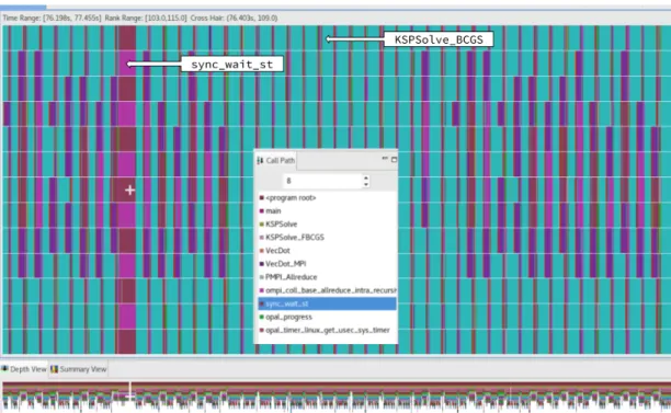
Initial data collection and analysis also revealed that HPCToolkit also collects information about MPI helper threads. I have in many cases excluded this data, but the data regarding functions like opal progress are included because these happen in the main thread of the program. Because several functions of interest were related to communication, trace data was collected for the largest case using 32 nodes, an example of which is shown in figure 3.1. Thesync wait stfunction that is shown in magenta and the purple ompi_coll_base_allreduce_intra_ recursivedoublingare both child items of PMPI Allreduce, and both then re-sult in calls toopal progress. The metrics in 3.1 related toopal progress can be considered an aggregate of these calls. The root of these calls toPMPI Allreduce can largely be associated with calls to IBTK::CCPoissonHypreLevelSolver:: solveSystemand KSPGMRESClassicalGramSchmidtOrthogonalization. Gram Schmidt Orthogonalization involves many dot products, which inherently re-quire a great deal of communication because of the nature of the operation requires a call to PMPI Allreduce which is a blocking MPI operation. Calls to SAMRAI::tbox::Schedule::communicate and SAMRAI::tbox::Schedule::

finalizeCommunicationoriginate fromIBTK::HierarchyGhostCellInterpolation:: fillData. These calls too eventually callopal progresswhile they wait for MPI

communication to complete.

The term “ghost cells” refers to the cells on the boundary of the patch that a rank is performing computations on. These ghost cells provide data access to cells that belong to a separate patch and may be “owned” by different MPI process. Use of ghost cells then necessitates MPI communication.

(25)

im-Figure 3.1: The trace shows that during calls toPMPI Allreducenot all ranks are left in function calls that indicate they are waiting. Rather, this waiting behavior is distributed in what appears to be a isolated region. This pattern is repeated throughout the trace.

balance, because the total amount of time any rank spent in either of these func-tions varies a good deal. The total time that anythread of the 32 node case spent in KSPGMRESClassicalGramSchmidtOrthogonalization is shown in figure 3.2, and the same metric is shown forIBTK::HierarchyGhostCellInterpolation:: fillData in figure 3.3. This graph is generated by HPCToolkit and graphs the metric of each thread, including the MPI helper threads. For example, the main thread of rank 2 is 2.0 and the two MPI helper threads are 2.1 and 2.2. Each of these helper threads have a dot plotted at 0 time spent in the function because these threads contain no calls from the main program. HPC-Toolkit reports that the standard deviation of the time that any rank spent in KSPGMRESClassicalGramSchmidtOrthogonalization for the 32 nodes case was 9.01×105 _{and for} _{IBTK::HierarchyGhostCellInterpolation::fillData} _the

(26)

Figure

3.2:

The

total

time

that

an

y

thr

ead

of

the

32

no

de

case

sp

en

t

in

KSPGMRESClassicalGramSchmidtO

rthogonalization

.

Some

main

threads

sp

en

t

almost

twice

as

long

in

the

call

as

(27)

Figure

3.3:

The

total

time

that

an

y

thr

ead

of

the

32

no

de

case

sp

en

t

in

IBTK::HierarchyGhostCellInter

polation::fillData

(28)

Increase in runtime in 32 node case relative to one node runtime

Function name Relative increase

opal progress 3.26E+00

SAMRAI::tbox::Schedule::finalizeCommunication 1.28E+00

SAMRAI::tbox::Schedule::communicate 9.00E-01

run example 4.42E-01

KSP PCApplyBAorAB 1.93E-01

PCApplyBAorAB 1.93E-01

IBTK::PETScKrylovLinearSolver::solveSystem 1.65E-01 IBTK::FACPreconditioner::FACVCycleNoPreSmoothing 1.49E-01

IBTK::FACPreconditioner::solveSystem 1.41E-01

Table 3.1: Results from weak scaling run of IBAMR application solv-ing ∆u = f repeatedly to gauge scalability of the linear solver used. The poorest scaling function call is a function called when MPI calls are waiting to complete, opal progress. This is a child item of both IBTK::HierarchyGhostCellInterpolation::fillData and KSPGMRESClassicalGramSchmidtOrthogonalization.

(29)

Figure 3.5: A log scale shows that the growth in the time spent in calls to opal progress scales much poorer than all other calls. Several communication intensive calls all end up calling opal progress to manage how long the rank should wait and when it can proceed past a barrier.

3.2 3D ABC Flow Simulation

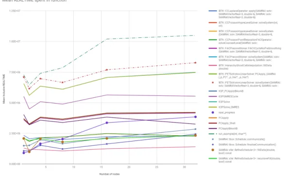
Initial analysis of the data from running the ABC flow simulation from IBAMR showed problematic behavior of a minor function, resetLevels1, which is called implicitly by objects of typeSAMRAI::math::HierarchySideDataOpsReal, a class used extensively in IBAMR. The average inclusive time forresetLevelsis shown in figure 3.6 in the red dotted line with stars at the collected data points in figure 3.6.

Investigation into the source code revealed that resetLevels performed aO(n2

patches)≥ O(n2

processes) operation (there is always at least one patch per process) that was

essentially a “no-op”, as it it made no meaningful change to the state of the program. The code loops over all the patches, of which there are at least as many as there are MPI processes running, or in our case, this is the same as the number of cores. Then for each patch it calls makeNonOverlappingBoxLists4, which itself is also loops over an array that is the size of all the patches. This set of nested loops is O(n2

patches), and it must be linear in order to weakly scale.

This is by nature of the fact that the number of patches will always be bounded below by the number of processors, so if any algorithm scales quadratically with the number of processors, the average time that it takes to complete will never

1_I _will _refer _to _{SAMRAI::math::HierarchySideDataOpsReal::resetLevels} _as

resetLevelsfor the remainder of the text.

4_{SAMRAI::hier::BoxUtilities::makeNonOverlappingBoxLists}_{, original source code}

(30)

Figure 3.6: Average inclusive time a rank spent in each function from initial profiling of the 3D Shear Flow simulation. NoticeresetLevels3, represented by the dashed line with stars at the data points, takes very little time in the 1 node case, and surpasses other main routines in the 32 node case. The vertical axis is in a log scale.

be constant, as is desired. Moreover, nothing of substance appeared to be done with this work!

Boyce Griffith supplied me with a patched version of SAMRAI whose sole dif-ference was to “comment out” this problematic code, effectively deleting it. The function was called in several related classes as well, and in the patched version was also effectively deleted with preprocessor statements that excluded it from being compiled. To confirm our hypothesis, I also instrumented SAMRAI with Score-P and rebuilt IBAMR and the application I was profiling. Previously, only resetLevelshad appeared the profiling data, but by instrumenting Score-P and inserting a custom user region inmakeNonOverlappingBoxesin both the patched and unpatched versions of SAMRAI,makeNonOverlappingBoxesappeared in the subsequent profiling data5

I performed the trials again, this time running the patched and unpatched versions in serial (one after the other) but in the same submission script given to the SLURM scheduler on the cluster, so they would run on the same hardware. Additionally, I had originally run the 32 node case with a base grid spacing of

N = 196, which cubed is not evenly divisible by the number of cores, 256. In the second run, I used the final configuration as is described on in the Methods section. I instrumented the patched SAMRAI in the same manner as the original SAMRAI, in case there were any other calls to makeNonOverlappingBoxes that were not excluded.

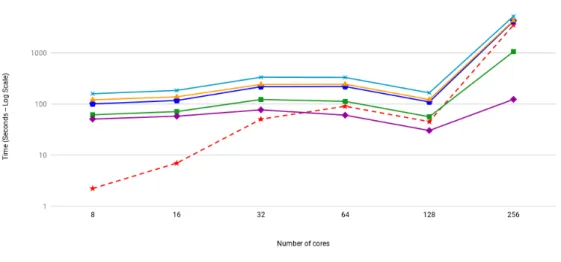
Figure 3.7 makes it clear that the calls to makeNonOverlappingBoxes make

5_{The instrumented version of}

(31)

Figure 3.7: Results from application using unpatched SAMRAI with Score-P instrumentation to expose timing of makeNonOverlappingBoxes

Comparison of average solve time (advanceHierarchy)

Cores Patched Unpatched Difference (seconds) Speedup Factor

8 135.87375 123.05625 -12.8175 ≈1

16 141.626875 140.385625 -1.24125 ≈1

32 206.913125 244.45 3.75E+01 1.2

64 167.1875 245.3125 78.125 1.5

128 203.125 538.28125 335.15625 2.7

256 305.078125 2046.875 1741.796875 6.7

Table 3.2: Speedup of IBAMR solve times gained by refactoring resetLevelsin SAMRAI

(32)

(33)

Chapter 4 Discussion

4.1 Interpretation of Results

4.1.1 3D Krylov Solver Results

Developing what a viable weak scaling trial was of the krylov method linear solver I was studying consumed a good deal of my time. First, I had to arrive at what parameter values for the IBAMR applications to use to produce the right kind of data to assess the weak scaling of the its constituent parts. Furthermore, I had the technical challenge of determining how to execute it, and finally how to process the data collected. This led me to engage a great deal of self education regarding using the cluster’s schedule manager, SLURM, using the module sys-tem for loading and unloading compilers, acquiring and building HPCToolkit’s dependencies, investigating the various options that each of HPCToolkit’s inter-faces take (hpcstruct, hpcrun, hpcprof, hpcprof-mpi), and attempting to decipher the hpcviewer and hpctraceviewer graphical user interfaces. I in-vested what was probably excessive time attempting to write scripts that would automate the entire process from end to end before I had performed the process interactively to a sufficient extent to understand what I needed to get out of the entire venture.

(34)

the program obfuscated the data and made it more difficult to identify problem areas in the program.

It does appear that the function calls posing the greatest blockers to scalability were internal MPI calls that are direct child items of function calls within the IBAMR program. The opal progress calls (distinct from the progress engine threads) belong to the OPAL interface that exposes a consistent interface to OpenMPI for accessing operating system and architecture dependent features such as memory, discovery of network interfaces, and access to system timers. The fact that the technology that IBAMR relies on to parallelize its tasks poses its greatest measured challenge to scalability in this example underlines the fact that no matter the efficiency of code implemented in IBAMR, it will never be more scalable than any such intensive use of MPI itself.

OPAL is a library that OpenMPI relies on to be portable across various architectures. Source: Open MPI by Jeffrey M. Squyres from The Architecture

of Open Source Applications [20]

If any action was to be taken from these results, it would have to be to attempt to reduce the amount of MPI communication, which is not a very clear directive. In conclusion, no clear prescriptions for performance improvement were drawn from this study, though many other lessons were learned about the underlying functioning of MPI programs and profiling software.

4.1.2 3D ABC Flow Simulation Results

This case study produced information that was much more intelligible upon first review, as there was a clear suspicious function call. It is my impression that the ability to filter the portion of the program studied helped me greatly to not get lost in great masses of information. If one function is called by many others, it can cause the inclusive time of many parent items in the call tree to appear large. It is imperative to find the lowest problematic item in the call stack in order to isolate and resolve problematic code.

(35)

be larger for runs that used more nodes and processors. While it is hazardous and unwise to make statements about the exact runtime of non instrumented, optimized code, it is clear that general trend of IBAMR simulation using the patched SAMRAI exhibits much better weak scaling.

This positive experience with using Score-P may be misconstrued as transfer-able to studying other applications. What is the case is that when you have access to a working Score-P compiler collection for the the set of compilers that you are using, Score-P provides some good features for cutting down on the flood of data and some reasonable data presentation software. Getting to that point of having a compatible Score-P installation can pose challenges that were not exhibited by this particular study, and it should be kept in mind that each and every Score-P application must be rebuilt if the compilers are rebuilt. Additionally, users must be very aware of various environment variables and their shell’s$PATHbecause Score-P relies on many environment variables to configure it at runtime, which can yield scenarios where it is not clear to the user what the current configuration of Score-P is.

4.2 Technical Limitations

A limiting factor for doing this scaling study was fitting jobs within the con-straints of the rules of the job scheduler on the cluster. Collecting data from a trial using 64 nodes would have made the data set much more robust, but con-figuration limitations prevented this. This was not possible because there are separate partitions that SLURM allows the jobs to be run on. It happened to be the case that I was not allowed to run a job using 512 cpus on the partition that is named “528” after the fact that it has 528 cores on it, because I also wanted 64 nodes and for the entire time period in which I was conducting this study, some number of nodes had been removed from the partition for maintenance, preventing users from using that number of nodes. This was only discovered af-ter contacting the the system administrators when job submissions that seemed well formed were rejected by the schedule manager. The next partition size is “2112” and has 96 nodes, but requires you to use at least 529 cores in any one job! Despite petitioning the system administrators several times, I was never able to get past this configuration issue.

Dogwood Partition Sizes and User Limits (Per Job)

Partition Name # Nodes Min # cores Max # cores

528 queue 87 45 528

2112 queue 96 529 2112

16764 queue 183 2113 16764

debug queue 87 none 88

cleanup queue 87 none 4

Source: UNC ITS Research Help pages [21]. While at peak capacity the 528 queue has 87 nodes, during the duration of this study the cluster was under

(36)

4.3 User experience of Profiling Tools

4.3.1 Score-P

Score-P worked “out of the box” in my initial configuration using gcc and

g++ 4.8.5 with OpenMPI, which was a positive experience. Later attempts to build Score-P on other systems and with other compilers revealed its dependen-cies on Qt libraries, which are graphical libraries that are not always available on “headless” servers that are exclusivly accessed via ssh sessions. This is be-cause Score-P chooses to build its graphical interface as a standard part of its build despite the fact that it is software meant to run on systems that often not often offer a windowing system. Furthermore, while it uses an autotools based configure script, it makes non-standard use of its options. For example, the script provides an option, --without-cube, cube being the name of the graphi-cal user interface. Suprisingly, use of this option does not build Score-P “without” cube. Instead, it indicates that the user does not have any pre-existing copy of cubefor Score-P to use, in which case it builds a bundled version of cube. This type of abuse of language, while common, is still offensive. Attempts to compile Score-P with more modern versions of gcc, including a version of gcc 6 failed to compile due to problems that appeared to be related to the more strict in-terpretations of the C++ standards implemented in more recent version of the GNU compiler collection [22]. This is also not uncommon, many libraries still fail to be C++11 compliant, even though gcc 6 moved to the C++14 standard and the current development version of the GNU compiler collection is version 8. These serious portability and compatibility issues make the fact that you must build Score-P for every compiler collection that you may use a perilous task if the researcher is responsible for building and maintaining the Score-P software collection themselves.

These criticisms aside, since I was fortunate enough to have a working instal-lation for the duration of the study of the 3D ABC flow simuinstal-lation, I was able to collect data and analyze it. This analysis yielded very useful information. The ability to scope the data collection using user defined regions and the filter file allowed me to cut down on the size of the profile collected, which kept the data sets for my experiments at a very reasonable size. Beyond file size considerations, any ability to reduce the amount of “noise” that the user has to sort through in order to find information of interest is highly valuable.

I did find the cube graphical interface relatively easy to use and understand and did not experience any failures of the software to function as advertised. Once the data was imported into the cube viewer, sorting options were hidden from plain view. Options to sort function calls on their metrics are discovered by right-clicking in a certain region of the display. This is not obvious, but useful and easy once found. There was no search function, but selection of a function call in the context tree view also selected in in the flat view, and the opposite case worked as well, which helped identify whereresetLevelswas being called. The break down of metrics over switches and nodes also provided good insight into load balance and the network topology of the nodes provisioned for a job.

(37)

compare the effects of certain optimization strategies, Cube includes a feature de-signed to simplify cross-experiment analysis.” This feature is not named in the help text. Further investigation revealed the existence of another command line tool built when cube is built called cube cmp [23], but it is not usable for weakscaling type trials because it requires that they be run on identical “system dimensions”, a phrase used to describe the number of MPI ranks.

There is no data export option in the graphical interface of cube but there is an additional command line tool called cube dump which is advertised as being able to export to csv, gnuplot, and a binary data format understood by the statistical programming language R [23]. I never investigated this because I chose to do the simplest and fastest thing I could do to get any insight on the weakscaling of the program, which was to simply copy values from the screen onto a spread sheet.

In summary, the Score-P toolkit is a feature rich toolkit that can be used to gain significant insight into the performance of parallel codes, and exhibits many of the same portability, compatibility, and usability problems that beset most scientific software.

4.3.2 HPCToolkit

HPCToolkit, once built, can be used to run and measure any application, regardless of how it was compiled. For this reason, I only ever built HPCToolkit once, so I cannot attest to its compatibility with various tool chains. The fact that I, as a user, do not have to worry about rebuilding this tool if my envi-ronment changes is in and of itself very valuable. Additionally, all components of the HPCToolkit environment are free, which is a major consideration if the researcher wants to analyze the trace data of a program and the institution they are affiliated with does not have a license for Vampir. Even if the funds can be made available, the process of obtaining funds itself takes valuable resources, and if the researcher themselves must make this petition for funds, the process of obtaining funds stands in direct competition for the researcher’s time that may have been spent getting results. Other positive elements to using HPCToolkit includes an active and responsive mailing list that puts users in direct contact with the core developers. These core developers are also productive writers and have many easily found publications and presentations available to augment the official documentation available on the HPCToolkit website.

The multiple stages that the data must go through to produce a usable data set makes the workflow relatively complicated and fragile to script. The fact that the

hpcprof and hpcprof-mpi were intermittently unreliable produced situations in which it was unclear what state the data was in if some of the processing was done in the job submission script along with the simulation.

Given a well formed database, I found using the profile viewer hpcviewer

(38)

metrics that pull data from multiple databases. Another challenge is the inter-mingling of the MPI theads into the data of the main program. This makes some of the metrics HPCToolkit calculates for the user of questionable use, because in the case of the experiments I ran, two thirds of the threads never spent any time in the function calls of interest, skewing the data for some metrics on the order of 10×107. There is an ability to filter based on the threads, but this removes the columns of the metrics of interest from the view.

To summarize, HPCToolkit offers the user a good deal of information that they may be able to use to help them identify problem areas in their code. It avoids many compatibility issues by using the sampling approach as opposed to instrumentation. The sheer amount of data and the possibly non-obvious intermixing of data about different threads poses challenges to the user’s ability to understand the data collected. Proficient use of HPCToolkit requires the user to educate themselves about various hardware counters function and meaning, and to understand more about the inner workings of the MPI implementation they are using.

4.4 Conclusion

I stand with my ethic professed in the methods section that it is in the interest of a programmer investigating the performance of their program to take routes of least resistance when it comes to tool selection and data analysis. This said, this method of “quickest returns” should not be confused with the method of “most rapid change of tools to avoid problems”. It is the aspiration of the programmer to make decisions about their tools and workflow that render an arrival at results that inform positive improvement of their program that yeilds a “path to solu-tion” in the manner of the paths taken by the steepest descent method of root finding in figure 4.1 parts (a), (c), or (d). Rapid changes in tool selection and workflow may yield a path more akin to figure 4.1 part (b) however. Any change of tool set or method incurs overhead and this itself delays arrival at any results that may inform action. While the programmer may wish for some tool-set that will save them from having to learn any details of how the network and hardware infrastructure they use works or the performance and implementation of the li-braries they rely on, this level of abstraction is not currently available nor do I hypothesize that it will become available in any reasonable time scale.

The poor performance identified in the resetLevels method in SAMRAI was perhaps the easiest type of problem to identify, and the resolution to the problematic code yielded easily measurable benefits. This class of problem that only exhibits itself at scale and involves intensive computation that scales in some super-linear fashion in proportion to the number of CPU cores is easily noticed when data in plotted in the fashion of figure 3.6. In smaller runs, resetLevels took very little time, and only behaved problematically for the larger scaled runs. These types of problems are not likely to be noticeable to developers running their code on a local machine for testing, but are very noticeable in a weak scaling study of this kind.

(39)

Figure 4.1: Paths the steepest descent method will take given differently con-ditioned problems and initial guesses. Source: “Conjugate Gradient Method Without the Agonizing Pain”, Figure 18. [24]

to complete to proceed. While I was not able to produce any concrete recom-mendation as to a course of action to deal with the behavior of the several parent calls to opal progress, including the Gram Schmidt orthogonalization routine and the Ghost Cell filling operation, I do believe that this problem would be best pursued by continued analysis of the trace data. This gives a good argument for the use of profiling software that the researcher can visualize the trace data format.

(40)

Bibliography

[1] J. Chang, K. B. Nakshatrala, M. G. Knepley, and L. Johnsson, “A performance spectrum for parallel computational frameworks that solve pdes,” CoRR, vol. abs/1705.03625, 2017. [Online]. Available: http://arxiv.org/abs/1705.03625

[2] A. N. Laboratory, “The portable, extensible toolkit for scientific computation,” 2018, [Online; accessed 27-February-2018]. [Online]. Available: https://www.mcs.anl.gov/petsc/

[3] L. L. N. Laboratory, “Samrai: Structured adaptive mesh refinement application infrastructure,” 2018, [Online; accessed 27-February-2018]. [Online]. Available: https://computation.llnl.gov/projects/samrai

[4] S. in the Public Interest, “Open mpi : Open source high performance computing,” 2018, [Online; accessed 27-February-2018]. [Online]. Available: https://www.open-mpi.org/

[5] A. N. Laboratory, “Mpich: A high-performance, portable implementation of mpi,” 2018, [Online; accessed 27-February-2018]. [Online]. Available: http://www.mcs.anl.gov/project/ mpich-high-performance-portable-implementation-mpi

[6] A. S. Almgren, “Introduction to block-structured adaptive mesh re-finement (amr),” 2018, [Online; accessed 27-February-2018]. [On-line]. Available: http://hipacc.ucsc.edu/Lecture%20Slides/2011ISSAC/ AlmgrenHIPACC July2011.pdf

[7] I. Free Software Foundation, “The libunwind project,” 2018, [Online; accessed 27-February-2018]. [Online]. Available: http://www.nongnu.org/ libunwind/

[8] P. A. P. Interface, “Papi : Performance application programming interface,” 2018, [Online; accessed 27-February-2018]. [Online]. Available: http://icl.cs.utk.edu/papi/index.html

[9] J. MellorCrummey, “Performance analysis of mpi+openmp programs with hpctoolkit,” 2018, [Online; accessed 27-February-2018]. [Online]. Available: http://hpctoolkit.org/slides/hpctoolkit-og15.pdf

(41)

[11] R. University, “Hpctoolkit is an integrated suite of tools for measurement and analysis of program performance,” 2018, [Online; accessed 27-February-2018]. [Online]. Available: http://hpctoolkit.org

[12] V. I. H. P. SUPERCOMPUTING, “Scalable performance measurement infrastructure for parallel codes,” 2018, [Online; accessed 27-February-2018]. [Online]. Available: http://www.vi-hps.org/projects/score-p/

[13] G.-T. GmbH, “Vampir performance optimization,” 2018, [Online; accessed 27-February-2018]. [Online]. Available: https://www.vampir.eu/

[14] J. Brown, M. G. Knepley, and B. F. Smith, “Run-time extensibility and librarization of simulation software,” CoRR, vol. abs/1407.2905, 2014. [Online]. Available: http://arxiv.org/abs/1407.2905

[15] J. Stuecheli12 and L. K. John, “Cache capacity and memory bandwidth scaling limits of highly threaded processors,” 2009.

[16] J. MellorCrummey, “Hpctoolkit users manual,” 2017, [Online; accessed 27-February-2018]. [Online]. Available: http://hpctoolkit.org/manual/ HPCToolkit-users-manual.pdf

[17] A. Z. Jack Xin, Yifeng Yu, “Periodic orbits of the abc flow with a=b=c=1,” ArXiV, Tech. Rep. arXiv:1601.02724, 2016. [Online]. Available: http://lanl.arxiv.org/abs/1601.02724

[18] hpctoolkit [email protected], “Hpctoolkit performance tools: hpcviewer and hpctraceviewer graphical user interfaces,” 2018, [On-line; accessed 27-February-2018]. [Online]. Available: https://github.com/ HPCToolkit/hpcviewer

[19] Google, “Vlookup,” 2018, [Online; accessed 27-February-2018]. [Online]. Available: https://support.google.com/docs/answer/3093318?hl=en

[20] J. M. Squyres, “Open mpi,” 2018, [Online; accessed 27-February-2018]. [Online]. Available: http://www.aosabook.org/en/openmpi.html

[21] [email protected], “Dogwood partitions and user limits,” 2018, [Online; accessed 27-February-2018]. [Online]. Available: https://help.unc.edu/help/ dogwood-partitions-and-user-limits/

[22] the GCC team, “Porting to gcc 6,” 2018, [Online; accessed 27-February-2018]. [Online]. Available: https://gcc.gnu.org/gcc-6/porting to.html

[23] Scalasca, “Cube user guide,” Unknown, [Online; accessed 27-February-2018]. [Online]. Available: https://apps.fz-juelich.de/scalasca/releases/cube/4.3/ docs/manual/userguide.html

(42)

Appendix A: Original resetLevels

1 t e m p l a t e<i n t DIM, c l a s s TYPE>

2 v o i d H i e r a r c h y S i d e D a t a O p s R e a l<DIM, TYPE>: : r e s e t L e v e l s (

3 c o n s t i n t c o a r s e s t l e v e l ,

4 c o n s t i n t f i n e s t l e v e l )

5 {

6 i n t i ;

7 #i f d e f DEBUG CHECK ASSERTIONS

8 TBOX ASSERT ( ! d h i e r a r c h y . i s N u l l ( ) ) ;

9 TBOX ASSERT( ( c o a r s e s t l e v e l >= 0 )

10 && ( f i n e s t l e v e l >= c o a r s e s t l e v e l )

11 && ( f i n e s t l e v e l <= d h i e r a r c h y−>g e t F i n e s t L e v e l N u m b e r ( ) ) ) ;

12 #e n d i f

13

14 d c o a r s e s t l e v e l = c o a r s e s t l e v e l ;

15 d f i n e s t l e v e l = f i n e s t l e v e l ; 16

17 f o r (i n t d = 0 ; d < DIM ; d++) {

18 d n o n o v e r l a p p i n g s i d e b o x e s [ d ] . r e s i z e A r r a y ( d f i n e s t l e v e l +1) ;

19 }

20

21 f o r (i n t l n = d c o a r s e s t l e v e l ; l n <= d f i n e s t l e v e l ; l n ++) {

22 t b o x : : P o i n t e r< h i e r : : P a t c h L e v e l<DIM> > l e v e l = d h i e r a r c h y−>g e t P a t c h L e v e l ( l n ) ;

23 h i e r : : BoxArray<DIM> s i d e b o x e s ;

24 c o n s t i n t n = l e v e l−>getNumberOfPatches ( ) ;

25

26 f o r (i n t nd = 0 ; nd < DIM ; nd++) {

27 s i d e b o x e s = l e v e l−>g e t B o x e s ( ) ;

28 f o r ( i = 0 ; i < n ; i ++) {

29 s i d e b o x e s [ i ] =

30 pdat : : SideGeometry<DIM>: : t o S i d e B o x ( s i d e b o x e s [ i ] , nd ) ;

31 }

32 h i e r : : B o x U t i l i t i e s<DIM>: : m a k e N o n O v e r l a p p i n g B o x L i s t s (

33 d n o n o v e r l a p p i n g s i d e b o x e s [ nd ] [ l n ] ,

34 s i d e b o x e s ) ;

UNC_Bachelor_Thesis_in_Mathematics.pdf

Assessing the Scalability of Parallel

Programs: Case Studies from IBAMR

Elijah DeLee

Abstract

Contents

Chapter 1

Introduction

1.1

Defining scalablity

1.2

Challenges to scalability

1.2.1

MPI Communication Overhead

1.3

Problem size

1.4

Formative Assessment of Performance

Chapter 2

Methods

2.0.1

Methods to gain introspection

2.0.2

Presentation and Analysis of the data

2.1

Tool Selection

2.2

Preparing the weak scaling trials

2.2.1

Case Study 1: Linear Solver with HPCToolkit

2.2.2

Case Study 2: 3D ABC Flow with Score-P

2.3

Data Analysis

2.3.1

HPCToolkit Data

2.3.2

Score-P Data

Score-P data analysis workflow

Chapter 3

Results

3.1

Krylov Linear Solver

3.2

3D ABC Flow Simulation

Chapter 4

Discussion

4.1

Interpretation of Results

4.1.1

3D Krylov Solver Results

4.1.2

3D ABC Flow Simulation Results

4.2

Technical Limitations

4.3

User experience of Profiling Tools

4.3.1

Score-P

4.3.2

HPCToolkit

4.4

Conclusion

Bibliography

Appendix A: Original resetLevels