Real Time Motion Vector Extraction of Moving Objects From Video Images

Real Time Motion Vector Extraction of Moving Objects From Video Images

Mahir Serhan TEMİZ1,

Usak University, Faculty of Engineering, Department of Geomatic Engineering, Usak, Turkey.

Sedat Doğan2,

Ondokuz Mayıs University, Faculty of Engineering, Department of Geomatic Engineering, Samsun, Turkey.

Abstract

The use of video images is rapidly growing from day to day to provide automation such as moving objects and extraction of their motion orbits. Object tracking by analyzing motion and shape in video gains more attractions in many computer vision applications including video

surveillance, motion analysis and extraction for computer animation.In order to track moving

objects with video images, points to be tracked which belong to the object on the successive video frames, should be selected automatically. In this paper, detailed studies have been performed for extraction of motion vectors. In order to track moving objects from video images, the points to be tracked which belong to the moving object on the successive video frames should be selected automatically. For this purpose we use corner detection algorithms to automatically select those points. For tracking of the selected points we use Lukas – Kanade (LK) Optical Flow approach

Keywords: Motion orbits, Optical Flow, Image Pyramid, LK Optical Flow.

INTRODUCTION

Using of video sequences are increasing in several applications for automation, for instance tracking moving objects, extracting trajectories, finding traffic intensity or estimating vehicle velocity etc.

Motion vector estimation is an important parameter for video segmentation. Optical flow is the distribution of apparent velocities of movement of brightness patterns in an image. Optical flow can arise from relative motion of objects and the viewer. Consequently, optical flow can give important information about the spatial arrangement of the objects viewed and the rate of change of this arrangement. Discontinuities in the optical flow can help in segmenting images into regions that correspond to different objects (Tamgade and Bora, 2009).

1994).

In order to track moving objects from video images, the points to be tracked which belong to the moving object on the successive video frames should be selected automatically. For this purpose we use corner detection algorithms to automatically select those points.

In the literature, generally two methods are used for tracking the selected points. Maduro et al. (2008), have used Kalman filtering method for tracking points on the subsequent frames to estimate the velocities of the vehicles, and they have reported 2% accuracy. In the similar manner, Li-Qun et al. (1992), Jung and Ho (1999), Melo et al. (2004) and Hu et al. (2008b) have also used the Kalman filtering method for tracking the selected points. The other method used for tracking the selected points is optical flow. Sand and Teller (2004), Sinha et al. (2009), Doğan et al. (2010) and Santoro et al. (2010), have used optical flow method for tracking points in subsequent frames.

There have been various researches for video-based object extraction and tracking. One of the simplest methods is to track regions of difference between a pair of consecutive frames, and its performance can be improved by using adaptive background generation and subtraction. Although the simple difference-based tracking method is efficient in tracking an object under noise-free circumstances, it often fails under noisy, complicated background (Shin et. al.2005). For tracking of the selected points we use Lukas – Kanade (LK) Optical Flow approach. During the real time tracking, some selected points may not be seen on the next frame. This situation may arise because of different reasons. Especially, when the vehicle is entering into or exiting from the FOV of the camera, the possibility of occurrence of this situation is too high. In order to prevent such situations, we have interpreted the algorithm with the image pyramid approach, which uses coarse to fine image scale levels.

IMAGE PYRAMID

Let us define the pyramid representation of a generic image I of size nx*ny. Let I0 = I be the

“zeroth" level image. This image is essentially the highest resolution image (the raw image). The image width and height at that level are defined as n0x = nx and n0y = ny. The pyramid

representation is then built in a recursive fashion: compute I1 from I0, then compute I2 from I1, and so on... Let L = 1, 2,… be a generic pyramidal level, and let IL-1 be the image at level L-1.

Denote nL-1x and nL-1 y the width and height of IL-1. The image IL-1 is then defined as follows:

IL (x,y)= 1/4 IL-1 (2x,2y) +1/8[IL-1(2x-1,2y)+IL-1(2x+1,2y) +IL-1(2x,2y-1)+ IL-1(2x,2y+1)] +1/16[IL-1(2x-1,2y-1)

+IL-1(2x+1,2y+1) +IL-1(2x1,2y+1) +IL-1 (2x+1,2y+1)] (1)

For simplicity in the notation, let us define dummy image values one pixel around the image IL-1 . for 0≤2x≤ nx L-1-1 & 0≤2y≤ nyL-1-1.

Therefore, the width nxL and height nyL of IL are the largest integers that satisfy the two

conditions:

nxL ≤ (nxL-1+ 1) /2 , (2)

Equations (1), (2) and (3) are used to construct recursively the pyramidal representations of the two images;

I & J:{ IL }L=0,……,Lm & { JL }L=0,……,Lm . (4)

The value Lm is the height of the pyramid . (Tamgade and Bora, 2009).

For details of the image pyramid approaches we refer the reader to (Bouget, 2000) and (Bradsky and Kaehler, 2008).

Automatic Selection of Points to be Tracked

In order to track moving objects with video images, points to be tracked which belong to the object on the successive video frames, should be selected automatically. It is well known that good features to be tracked are corner points which have large spatial gradients in two orthogonal directions. Since the corner points cannot be on an edge (except endpoints), aperture problem does not occur. One of the most frequently used definitions of a corner point is given in (Harris and Stephens,1988). This definition defines a corner point by a matrix which is xpressed by second order derivatives. These derivatives are partial derivatives of pixel intensities on an image and are ∂2x, ∂2y and ∂x∂y. By computing second order derivatives of pixels of an image, a

new image can be formed. This new image is called “Hessian image”. The name “Hessian” arises from the Hessian matrix that is computed around a point (Doğan, et. al, 2010). The Hessian matrix in 2D space is defined by:

(5)

Shi and Tomasi (1994), suggest that a reasonable criterion for feature selection is for the minimum eigenvalue of the spatial gradient matrix to be no less than some predefined threshold. This ensures that the matrix is well conditioned and above the noise level of the image so that its inverse does not unreasonably amplify possible noise in a certain critical directions.

When it is desired to extract precise geometric information from the images, the corner points should be found within a sub-pixel accuracy. For this purpose, the all candidate pixels around the corner point can be used. By using the smallest eigenvalues at those points, a parabola can be fitted to represent the spatial location of the corner point. The coordinates of the maximum of the parabola is assumed to be the best location for being a corner. Thus the computed coordinates are obtained in subpixel precision (Doğan, et. al, 2010).

   

 

   

 

   



 

 



2 2 2

2 2 2

y I x y

I

y x

I x

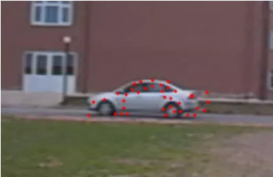
Fig -1: Automatically Selected Points

In our system, as soon as the camera begins for image acquisition, points are selected continuously in real time from the frame images. Fig-1 shows automatically selected points. On the first frame, points are selected and on the next frames those points are tracked and instantaneous velocity vectors of those points are computed.

Tracking of Selected Points

For estimation of motion vectors, correspondence of each selected point on the first frame on which the object appears for the first time, must be found on the next (successive) frame. In the ideal case, correspondence of a selected point must be the same point on the next frame. In order to find the corresponding point, there is no prior information other than the point itself. If we assume that each image in the each frame is flowing by the very short time period and thus changing the position during the flow, then a modelling approach which models this flow event can be used. These kinds of flow models are called “optical flow”.

Lukas-Kanade (LK) Optical Flow Method

When only one video camera is used, there is no information other than themselves of the selected points to find their correspondences on the next frame. For this reason, it is not possible to know exactly where the corresponding points are on the next frame. But however, by investigating the nature of the problem, some assumptions may be made about the possible locations where the corresponding points might be located. In order to ensure these assumptions are as close to the physical reality as possible, there must exist a theoretic substratum at which these assumptions are supported. Furthermore, this theoretic substratum must be acceptable under some certain situations. Lukas and Kanade have cleverly given three assumptions for the solution of the correspondence problem in their paper (Lukas and Kanade, 1981). The assumptions of Lukas-Kanade Method are:

1. Intensity values are unchanged: This assumption asserts that the intensity values of a selected point p(t) and its neighbours on the frame image I(t), do not change on the next

that really the possibility of the occurrence of this assumption is too high. Because, in a very short time period which is measured in milliseconds, the effects such as the lighting conditions of the scene medium etc. that cause the intensity values to be changed must not lead to meaningful change effects since the time is too short.

2. Location of a point between two successive frames changes by only a few pixels: The reasoning which the assumption is based on, is similar to the reasoning of the first assumption. Between the frame images I(t) and I(t + Δt), when Δt is getting smaller, then the displacement amount of the point also gets smaller. According to this observation, a point p(t) at (x,y) coordinates of image I(t) will be at the coordinates (x + Δx, y + Δy) on image I(t + Δt) and these new coordinates will be closer to the previous coordinates within a few pixels. Thus the positions of the corresponding points on both images will be very close to each other.

3. A point behaves together with its neighbours: The first two assumptions, which are assumed to be valid for a point must also be valid for its neighbours. Furthermore, if that point is moving with a velocity v, then its neighbours must also move with the same velocity v, since the motion duration Δt is too short.

The three assumptions above help develop an effective target tracking algorithm. In order to track the points and to compute their speeds by using the above assumptions, it is necessary to express those assumptions with mathematical formalisms and then velocity equations must be extracted by using these formalisms. For this purpose, the first assumption can be written in mathematical form as follows:

(6)

where I(p,t) is the intensity value of a point p on the image I(t) which was taken at the time instant t. Note that the geometric location of the point is expressed by its position vector p Є R2

(i.e., in 2D space). Here I(p,t) expresses the intensity value of a pixel at the point p on the frame image I(t). In similar way, the right side of the equation expresses the intensity value of the corresponding pixel at the point p + Δp on the frame image I(t + Δt). Accordingly, Equation (2) says that the intensity value of the point p on the current image frame does not change during the time period Δt that passed. In other words, it expresses that the intensity I(p,t) does not change by the time Δt. In the more mathematical sense, change rate of I(p,t) iz zero over the time period Δt. This last situation is formally written as follows:

(7)

If the derivative given in Equation (7) is computed by using the chain rule of derivative, we obtain: (8) Δt) t t), y, (x, l( t) t), y, (x,

l(p  p 

In Equation (8), the derivative I/pis spatial derivative at point p on the image frame I(t). Thus

it can be expressed byI/pI . We can write this expression in explicit form as follows:

j

I

i

I

j

y

l

i

x

l

I



















The derivative p(t)/tcan also be written in a more explicit form:

(10)

If Equation (10) is investigated carefully, it can easily be seen that the vector (x/t)iis equal to the velocity of the point p in the x-axis direction. In other words, it is the x component namely vx

component of the velocity vector v. In similar way, the vector (y/t)j is the y component

namely vy component of the velocity vector v. Now we can rewrite the Equation (10) as follows:

(11)

If again Equation (8) is investigated, it is seen that the derivative I/tIt expresses the

change rate of the intensity values at point p, between the frame images I(t) and I(t + Δt). Thus, Equation (8) can be rewritten as follows:

(12) where:

















I

I

I

and















V

V

V

Then Equation (12) can be written as:

(14)

The values of Ix, Iy and It in Equation (14) can easily be computed from the frame images. The

variables vx and vy are two unknown components of the velocity vector v and these are

respectively the components in the directions x and y axes of the image coordinate system. In Equation (14), we have two unknowns to be solved, but we only have one equation. Since only one equation is not enough for unique solution of the unknowns, at the moment it seems not

j t y i t x yj) (xi t t (t)            p j v i v v t (t) y x     p 0 I

I.V t 







y x y

x

_V

I

V

.

I

I

_





possible to solve these unknowns. In order to solve these two unknowns, we need more independent equations. For this purpose, the third assumption of the LK algorithm is used. That is, point p behaves together with its neighbours. So its neighbours must also satisfy the Equation (10). In other words, neighbour points (or pixels) of point p must move with the same velocity

v(vx,vy). According to these explanations, the same equations as (14) are written for 3 × 3 or 5 ×

5 neighbourhood of the point p. In this case, we totally have 9 or 25 equations with the same unknowns vx and vy. Now the unknowns can be solved with overdetermined set of Equations (14)

by using least squares or total least squares estimation method (Doğan, et. al, 2010).

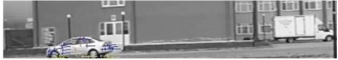
During the real time tracking, some selected points may not be seen on the next frame. This situation may arise because of different reasons. Especially, when the vehicle is entering into or exiting from the FOV of the camera, the possibility of occurrence of this situation is too high. In order to prevent such situations, we have interpreted the algorithm with the image pyramid approach, which uses coarse to fine image scale levels. Fig-2 shows estimated vectors.

Fig -2: Estimated vectors.

EXPERIMENTS AND RESULTS

In this paper, we propose a method for real-time estimation of the motion vectors of moving objects by using uncalibrated monocular video camera. Since it is not possible to extract 3D geometric information with one camera, in order to solve the speed estimation problem, some geometric constraints are required and the images should be taken under these constraints and the processing procedures should also be performed with those restrictions. For example, we assume that the imaged scene is flat. Perspective distortions on the acquired images must be either very small or of a degree that they can easily be rectified.

We have used a camera with a frame rate of 30 fps (frames per second) and with an effective area of 640 x 480 pixel2. The pixel size which corresponds to the effective area of the camera is 9 microns. The focal length of the camera is 5.9 mm. We capture images in grey level mode at 30 fps, meaning that a frame is captured within 33.3 milliseconds after the previous frame had been obtained. In order to solve the real time speed estimation problem, the authors have written a software system in C++ programming language. This software system has been used for all of the computations and test applications. Our software consists of two steps which contain offline and online operations, for details refer to (Doğan, et. al, 2010).

The rest of the operations are performed with our own codes written with Visual Studio C++ 2010. The total time of the operations takes about 30 milliseconds for our real time applications with a laptop computer (Intel Quad Core i7 2.6 Ghz CPU, 8 GB RAM).

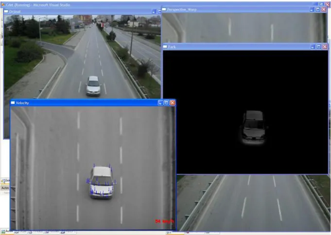
Fig-3 shows a general view of our software.

Fig -3: General view of our software.

REFERENCE

Barron, J.L., Fleet, D.J. and Beauchemin, S.S, 1994. Systems and Experiment Performance of Optical Flow Techniques, International Journal of Computer Vision, Vol.12:1, pp. 43-77

Bouget, J.Y., 2000. Pyramidal Implementation of the Lucas Kanade Feature Tracker Description of the Algorithm; Intel Microprocessor Research Labs: Santa Clara, CA , USA.

Bradsky G., and Kaehler A., 2008. Learning OpenCV Computer Vision with the OpenCV Library, O’Reilly Media, Inc, 555 p.

Doğan, S., Temiz, M.S. and Külür, S., 2010. Real Time Speed Estimation Of Moving Vehicles From Side View Images From An Uncalibrated Video Camera. Sensors. 10(5), pp. 4805-4824.

Harris C. and Stephens M., 1988. A Combined Corner and Edge Detector, Proceedings of the 4th Alvey Vision Conference, pp.147-151.

Hu, N., Aghajan, H., Gao, T., Camhi, J., Lee, C.H. and Rosario, D., 2008. Smart Node: Intelligent Traffic Interpretation, World Congress on Intelligent Transport Systems.

Jung, Y.K. and Ho, Y.S., 1999. Traffic Parameter Extraction Using Video-based Vehicle Tracking,

Li-Qun, X., Young, D. and Hogg, D.C., 1992. Building a model of a road junction using moving vehicles in: Hogg, D & Boyle,R.D. (editors) British Machine Vision Conference, pp. 443-452. Springer.

Lucas B.D., and Kanade T., 1981. An Iterative Image Registration Technique with an

Application to Stereo Vision, Proceedings of the 1981 DARPA Imaging Understanding Workshop,

pp. 121-130, Washington, USA.

Maduro, C, Batista, K, Peixoto, P. and Batista, J, 2008. Estimation Of Vehicle Velocity And Traffic Intensity Using Rectified Images, 15th IEEE International Conference on, Image Processing, pp. 777 – 780.

Melo J., Naftel A., Bernardino A., and Victor J.S., 2004. Viewpoint Independent Detection of Vehicle Trajectories and Lane Geometry from Uncalibrated Traffic Surveillance Cameras, Int. Conf. On Image Analysis and Recognition, 29 Sept.- 1 Oct., Porto, Portugal.

Sand, P. and Teller, S., 2004. Video Matching, ACM Transactions on Graphics (TOG), Vol. 22, No. 3, pp. 592-599.

Santoro, F., Pedro, S., Tan, Z.H. and Moeslund, T.B., 2010. Crowd Analysis by using Optical Flow and Density Based Clustering, 18th European Signal Processing Conference, Aalborg, Denmark, August 23-27.

Shi J., and Tomasi C., 1994. Good Features To Track, 9th IEEE Conference on Computer Vision and Pattern Recognition, pp. 593-600, Seattle, USA.

Shin, J., Kim, S., Kang, S., Lee, S.W., Paik, J., Abidi, B., Abidi, M., 2005: Optical flow-based real-time object tracking using non-prior training active feature model, Real-Time Imaging Vol:11, pp. 204–218.

Sinha, S., Frahm, J.M., Pollefeys, M. and Genc, Y., 2009. Feature Tracking and Matching in Video Using Programmable Graphics Hardware, Machine Vision and Application, Nov. 2009.

Biography of Authors

Mahir Serhan TEMİZ

Undergraduate: Ondokuz Mayis University / 2001 Master Degree: Ondokuz Mayis University / 2005 Doctorate: Istanbul Technical University / 2012 Assistant Professor: Usak University / 2003

Expertise : Photogrammetry, Image Processing

Sedat DOĞAN

Undergraduate: Karadeniz Technical University / 1994 Master Degree: Karadeniz Technical University / 1996 Doctorate: Istanbul Technical University / 2003 Assistant Professor: Ondokuz Mayis University / 2003 Associate Professor: Ondokuz Mayis University / 2015