KERNEL MACHINE METHODS FOR ANALYSIS OF GENOMIC DATA FROM DIFFERENT SOURCES
Ni Zhao
A dissertation submitted to the faculty of the University of North Carolina at Chapel Hill in partial fulfillment of the requirements for the degree of Doctor of Philosophy in
the Department of Biostatistics.
Chapel Hill 2014
Approved by:
Michael C. Wu
D Neil Hayes
Eric T Tchetgen
Wei Sun
c 2014 Ni Zhao
ABSTRACT
NI ZHAO: Kernel Machine Methods for Analysis of Genomic Data from Different Sources
(Under the direction of Michael C. Wu)
Comprehensive understanding of complex trait etiology requires examination of
mul-tiple sources of genomic variability. Recent advances in high-throughput biotechnology,
especially sequencing technology, have enabled multiple platform genomic profiling of
biological samples. In this dissertation, we consider using the kernel machine regression
(KMR) framework to analyze data from different genetic data sources.
In the first part of this dissertation, we develop a new strategy for identification
of large scale, global changes in methylation that are associated with environmental
variables or clinical outcomes via a functional regression approach. The density or the
cumulative distribution function of the methylation values for each individual can be
approximated using B-spline basis functions with the spline coefficients to summarize
the individual’s overall methylation profile. A variance component score test is proposed
to test for association between the overall distribution and a continuous or dichotomous
outcome and applied to two real studies.
In the second part, we construct a microbiome regression-based kernel association
test (MiRKAT) for testing the association between microbial community profiles and
a continuous or dichotomous variable of interest such as an environmental exposure or
disease status. This method regresses the outcome on the covariates (including
poten-tial confounders) and the microbiome compositional profiles through kernel functions.
We demonstrate the improved control of type I error and superior power of MiRKAT
In the final part, we focus on integrative analysis of genome wide association
stud-ies (GWAS) and methylation studstud-ies. We propose to use the KMR for first testing
the cumulative genetic/epigenetic effect on a trait and for subsequent mediation
anal-ysis to understand the mechanisms by which the genomic data influence the trait. In
particular, we develop an approach that works at the gene level (to allow for a
com-mon analysis unit across data types). We compare pair-wise similarity in trait values
between individuals to pair-wise similarity in methylation and genotype values, with
correspondence suggestive of association. For a significant gene, we develop a causal
steps approach to mediation analysis which enables elucidation of the manner in which
ACKNOWLEDGMENTS
My most sincere gratitude goes to my dissertation advisor, Dr Michael Wu, for
his guidance, understanding, patience, and most importantly, friendship during my
graduate studies. He encouraged and taught me to not only grow as a statistician but
also as an independent researcher. I should be thankful not only for his close guidance
and careful training through all of my dissertation topics , but also for his high spirit
and enthusiasm in academic studies. He managed to make my dissertation experience
both inspiring and enjoyable that I just feel that I have not learnt enough from him
yet.
Dr. Neil Hayes, among all my committee members, I had the longest working
relationship with him. I started working with him even before I joined the Department
of Biostatistics. I am grateful to work with him and get exposed to the cutting-edge
techniques and involved in some pioneering studies in cancer genomics. By setting an
great example as a world-class researcher, I learned enormously from him, not only
about cancer or genomics, but also about being a scientific researcher in the first place.
I was extremely delighted to work with Dr. Wei Sun for my master thesis, who has
been a motivating and encouraging mentor. The work with him has been an unique
experience which introduced me to different ideas and methods, both in the field of
genetics and statistics. I owe great gratitude to him for all the help he can possibly
offer.
I am greatly thankful to Dr. Yun Li for her encouragement and help when I
en-counter problems in my research. She has the warmest and most welcoming smile. I
personally consider her as a perfect combination of statistician and geneticist, from
I’d like to show my gratitude to Dr. Eric Tchetgen for reading a my dissertation
draft, offering special comments and suggestions, especially with respect to the causal
mediation analysis. I remembered the time when he kindly went through the effort the
derivation and proofs to help me evaluate one of our hypothesis when I went to Boston
to ask for help. I sincerely hope that I had more opportunities to work with him.
I would also like to thank my fellow students in the Department of Biostatistics,
for the friendship and the fun time we spend together, and all the members in the Neil
Hayes research group, especially Michele and Ashley, for being a welcoming academic
family and offering help whenever asked.
Finally and most importantly, I would like to thank my husband Xin Huang for all
these years of understanding, encouragement and unwavering love. He has been
instru-mental in instilling confidence in me, constitutes my source of comfort and courage, even
TABLE OF CONTENTS
LIST OF TABLES. . . x
LIST OF FIGURES . . . xi
1 Introduction . . . 1
2 Literature Review . . . 4
2.1 Multidimensional Genetic Data . . . 4
2.1.1 Genome Wide Association Study and Missing Heritability . . . 4
2.1.2 Gene Expression Data . . . 7
2.1.3 Metagenomics: Genomic Analysis of Microbial Communities . . 8
2.1.4 Epigenetics . . . 9
2.1.5 Group Based Analysis . . . 10
2.2 Semiparametric Model via Kernel Machine Regression . . . 13
2.2.1 Specification of h(Z) using Kernel Functions . . . 13
2.2.2 Estimation through Mixed Model Framework . . . 16
2.2.3 Variance Component Score Test . . . 18
2.3 Further Work on KMR in Genomic Studies . . . 19
2.3.1 KMR for Survival Outcomes . . . 19
2.3.2 Multivariate Phenotype Association by KMR . . . 21
2.3.3 Kernel Machine Test Under Multiple Candidate Kernels . . . . 22
2.4 Causal Mediation Analysis . . . 25
2.4.1 Regression Approach to Mediation . . . 25
2.4.3 Mediation Analysis in Genetic Analysis . . . 33
3 Global Analysis of Methylation via a Functional Regression Approach 35 3.1 Introduction . . . 35
3.2 Functional Estimation of Methylation Distributions . . . 38
3.2.1 Estimation of the Density for Each Sample . . . 38
3.2.2 Estimation of the Cumulative Distribution Function . . . 40
3.3 Variance Component Test in Approximated Distributions . . . 42
3.4 Simulations . . . 45
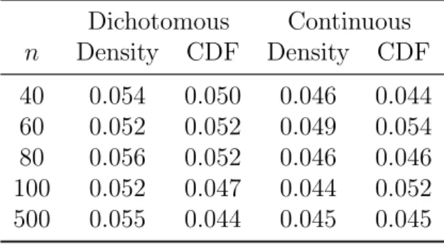
3.4.1 Type I Error . . . 45
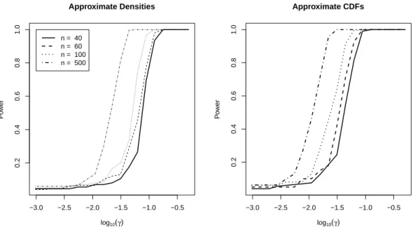
3.4.2 Power . . . 46
3.5 Data Applications . . . 47
3.5.1 Epigenetic Comparison of Newborns and Nonagenarians . . . . 47
3.5.2 Head and Neck Squamous Cell Carcinoma Methylation Study . 50 3.6 Discussion . . . 51
4 Microbiome Kernel Machine Profiling . . . 53
4.1 Introduction . . . 53
4.2 Methods . . . 55
4.2.1 Notation . . . 55
4.2.2 Distance Based Association Test for Microbiome Composition . 56 4.2.3 Microbiota Regression-based Kernel Association Test . . . 58
4.2.4 Optimal MiRKAT under Multiple Distance Metrics . . . 60
4.2.5 Numerical Experiments and Simulations . . . 61
4.3 Results . . . 62
4.3.1 Type I Error Control for MiRKAT and Competing Methods . . 62
4.3.3 Application to IBS and Smoking Data Sets . . . 64
4.3.4 Relationship between MiRKAT and Competing Methods . . . . 65
4.4 Discussion . . . 66
5 Integrative Analysis of Methylation and Genotyping Studies . . . . 70
5.1 Introduction . . . 70
5.2 Material and Methods . . . 73
5.2.1 Notation . . . 74
5.2.2 Cumulative Test of Genetic and Epigenetic effects . . . 74
5.2.3 Subsequent Mediation Analysis . . . 83
5.3 Simulations Study . . . 90
5.3.1 Simulation for Cumulative Test . . . 90
5.3.2 Simulation for Multivariate Causal Steps Model . . . 93
5.4 Results . . . 95
5.4.1 Empirical Size and Power for Cumulative Test . . . 95
5.4.2 Multivariate Causal Steps Model Results . . . 98
5.5 Discussion . . . 99
Appendix I: Exact Method for MiRKAT Using Multiple Kernels . . . 102
LIST OF TABLES
3.1 Type I error simulation results. . . 46
5.1 Cumulative Effect Tests Model Specification . . . 92
LIST OF FIGURES
2.1 Mediation Diagram . . . 26
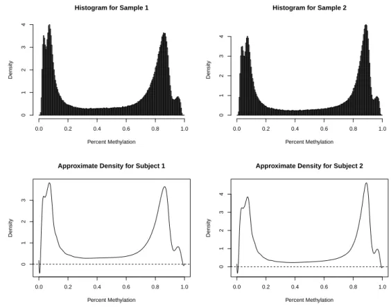
3.1 Approximating the density for each sample: Example histograms for two samples and the corresponding B-spline approximated densities. . . 41
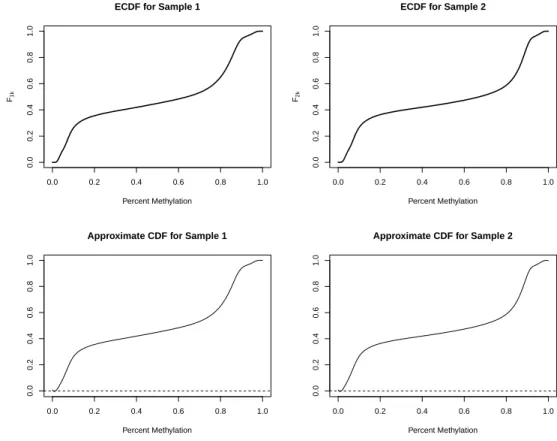
3.2 Approximating the CDF for each sample: example ECDFs for two sam-ples and the approximated B-spline approximations of the CDFs. . . . 43
3.3 Power simulations results. . . 48
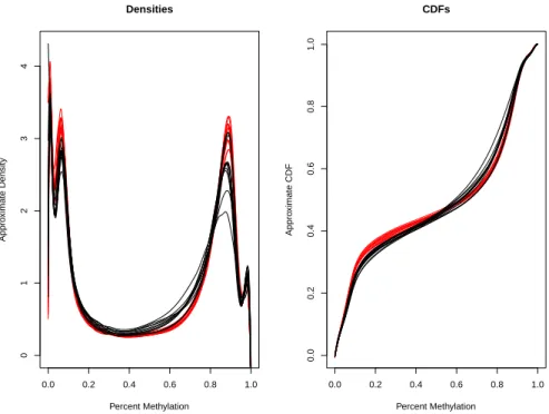
3.4 Approximate densities and CDFs from the nonagenarian study. Red curves are the nonagenarian methylation profiles and black curves are the infant methylation profiles. . . 49
3.5 Approximate densities and CDFs from the head and neck squamous cell carcinoma study. Red curves are the methylation profiles for the cancer cases and black curves are the methylation profiles for the healthy controls. . . 50
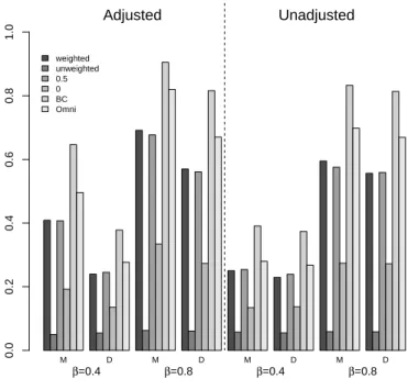
4.1 Type I error of different methods at α= 0.05 level: Data was simulated forn= 50 and only the 10 most abundant bacteria have any effect on the outcome. M: MiKRAT D: distance based method. ♦: nominal α= 0.05. 68 4.2 Power comparison of different methods: Data was simulated for n = 50
and only the 10 most abundant bacteria have any effect on the outcome. Additional covariates X and bacterial effect Z were simulated indepen-dently. M: MiKRAT D: distance based method. . . 69
5.1 Mediation Diagram . . . 84
5.2 Empirical Power for Tests on Cumulative Genetics and Epigenetic Effects 96
CHAPTER 1 Introduction
Complex diseases, such as cancer, cardiovascular disease, diabetes and Alzheimer’s
disease, which constitute the greatest public health burden both nationwide and
glob-ally, are considered to be caused by modest effects of multiple genes, interacting with
environmental and lifestyle factors. Comprehensive understanding of these complex
trait etiology requires examination of multiple sources of genomic variability.
Recen-t advances in high-Recen-throughpuRecen-t bioRecen-technology, especially sequencing Recen-technology, have
enabled multiple platform genomic profiling of biological samples, which can facilitate
the characterization of biological systems at multiple levels. For example, the Cancer
Genome Atlas (TCGA) project aims to generate comprehensive catalog of the genomic
changes of different cancers, including single nucleotide polymorphism (SNP), DNA
methylation, gene expression, microRNA expression, for the same set of tumor samples
(147, 148, 150). Similarly, the NCI60 project has profiled 60 human cancer cell lines
with respect to gene expression, protein expression, microRNA expression and drug
responses (221, 20, 178, 195, 182). Integrative analysis of these data sources promises
elucidation of the biological processes underlying particular phenotypes. Integrative
analysis of “multi-dimensional genomic data” has proven especially challenging.
Typ-ical analyses of large scale genomic data that examine each feature individually with
subsequent correction for multiple comparisons were problematic(198, 232). First,
corrections and the relatively smaller effect size in individual features. Further,
difficul-ty aries in interpretation and formation of biological hypothesis when too many features
are called significant. Finally, this method fails to capture the multi-feature/interative
effect and usually have poor reproducibility (223, 142).
To overcome many of these limitations, analysis that associate grouped features
with outcome has gained popularity during the recent years. For example, in Genome
Wide Association Studies (GWAS), multiple-SNP based analyses, in which multiple
related SNPs (by proximity to a gene, pathway or functional groups) are combined into
SNP set and jointly analyzed for association with outcomes of interest, have emerged
as a powerful alternative for identifying associations between multiple gene variants
and complex disease. Investigating cumulative effect of multiple related features (e.g
genes in a pathway, SNPs in a region or CpGs in a gene) across different platforms has
also become a ubiquitous strategy in different complex diseases(218, 94, 176, 240). One
particularly popular strategy in the multiple-feature association study is the kernel
ma-chine regression (KMR) test, which was initially proposed for gene expression data with
continuous or binary phenotypes(112, 111), but has also been extended to candidate
gene studies (96),case-control GWAS studies to test for SNP-set effect (229, 187, 139),
rare variants studies(230).
This approach is built upon a semi-parametric model within the kernel machine
regression framework (40) where the genomic effect can be modeled
nonparametrical-ly with simple confounding factors modeled parametricalnonparametrical-ly. Intuitivenonparametrical-ly, this approach
constructs a pairwise similarity matrix between genetic measurement through the use
of a kernel function, which can then be compared to the similarity between the
pheno-type of interest with high correspondence suggestive of association. Inference can be
conducted through the variance score test, which is operationally simple and fast as it
The dissertation is organized as follows. In Chapter 2, we review current literature
on analysis of multi-dimensional genetic data, with a focus on the KMR framework and
identify unsolved problems. In Chapter 3, we develop two related methodologies under
the KMR framework for identification of large scale, global methylation changes that
are associated with environmental variables, clinical outcomes or other experimental
condition. In Chapter 4, we extend this framework to the field of metagenomic studies
and develop methods for association between microbial composition and outcomes of
interest. In Chapter 5, we develop method to use the powerful kernel machine
frame-work for first testing the cumulative effect of both epigenetic and genetic variability on
a trait, and for subsequent mediation analysis to understand the mechanisms by which
CHAPTER 2 Literature Review
2.1 Multidimensional Genetic Data
Genetic research has undergone a dramatic transformation in the past decade
be-cause improved technology and reduced cost enabled collection of genetic data at
mul-tiple levels. Several large scale studies have collected multidimensional genomic data,
including but not limited to whole genome gene expression, genotyping, copy numbers
and rare variants; and have demonstrated the great potential of integrative analysis in
discovering the complex and interrelated biological foundation underlying disease
phe-notypes. While multidimensional genomic studies are gaining increasing popularity,
the methodology to perform the analysis has not kept pace with the collection of the
data.
In this section, we will review the commonly used methods in analyzing different
types of genomic studies and defer the KMR framework to Section 2.2
2.1.1 Genome Wide Association Study and Missing Heritability
Proposed almost 20 years ago as a potentially powerful approach to unravel the
genetic basis of complex diseases (163), genome-wide association studies (GWAS) have
become one of the most common tools for investigating the genetic architecture of
variant”, hypothesizing that complex diseases are at least partially attributable to
common variants present in more than 1−5% of human population (35, 161, 157). Facilitated by the commercially available “SNP chips” which capture most, although
not all, common variants in the genome, GWAS aim to detect association between
common variants (especially in SNPs) and disease phenotypes. GWAS have reported
hundreds of SNPs that are robustly associated with common phenotypes (133), some of
which the biological basis have successfully been elucidated (67, 48, 92) or have shown
clinical importance towards personalized medicine (37).
Typically, SNPs discovered by GWAS confer relatively small increments in risk
and can together account for only a small fraction of the genetic variation of complex
traits in human populations, leading to the perceived problem of missing heritability
(130, 134). A number of explanations have been suggested for this missing heritability,
including the existence of unmodeled epistatic interactions, the effect of rare variants
(157) and inherited epigenetic factors (83, 84).
Current GWAS usually test association between SNPs with a phenotypic trait, one
at a time, with stringent genome-wide adjustment for multiple testing. This procedure
can be underpowered due to a number of reasons. First, the effect size of individual
SNPs can too small to reach the genome-wide significance in GWAS(101). Secondly, the
true causal variants are rarely genotyped in practice and detection of association rely on
the linkage disequilibrium (LD) between genotyped SNPs and the causal variant. If the
LD was not sufficient between the causal variant and SNPs that are genotyped on the
GWAS platform, the power of detecting the true association will be reduced (101). This
can also cause the problem of poor reproducibility: many of the highly ranked SNPs
in the discovery phase of GWAS are false positives and cannot be validated because
the estimated association is not for the true causal SNP but the genotyped surrogate
Methods that consider joint effect of multiple SNPs simultaneously can be
advan-tageous because it reduces the total number of tests (hence the number of multiple
comparisons) and approximates the causal effect more effectively than could single
S-NP analysis (175). Moreover, the individual SS-NP approach considers only the marginal
effect of each SNP and fails to accommodate epistatic interaction effect between SNPs
(57), which have been shown to be ubiquitous to a number of common human
dis-eases (142), including type I/II diabetes (202, 39), inflammatory bowel disease (33)
and Alzheimer’s diseases (23, 36, 36). Testing for the epistatic effect e.g. gene-gene
interaction, is generally challenging because of the large number of potential
interac-tions (78). Alternative approaches that use prior biological information to form SNP
set and test for association between the SNP set and phenotypic traits are successful
in improving power and increase the heritability estimates (235, 63).
Rare genetic variants, alleles with a frequency less than 1−5% but potentially higher
penetrance, can be essential in influencing complex disease and constitute another
source of the missing heritability (179). Because of the relatively lower frequency,
rare variants are less likely to be captured by the conventional genotype platforms
used in GWAS. The advent of new sequencing technique (135) offers unprecedented
opportunities for assessing the contribution of rare genetic variation to complex diseases
(50). Standard methods that test for association with single markers are no longer
applicable unless the sample size and/or the effect size are extremly large (102, 128).
Methods analyzing rare variants involve testing the grouped/cumulative effect for a
set of markers across a genomic region, including the burden test and its derivatives
2.1.2 Gene Expression Data
Gene expression determines a variety of cellular phenotypes. Gene expression
pro-filing, which measures the activity/expression of thousand of genes simultaneously, has
been a routine practice in genetic studies since the microarray technology (212). More
recent technologies such as high-throughput RNA sequencing enables not only more
accurate determination of gene expression level (145), but structural variations, such
as allele-specific expression (167).
The primary goal of many gene expression studies is to identify genes that are
differ-entially expressed under two or more treatment conditions. Traditionally, differential
expression was assessed through fold change, t-test or ANOVA one gene at a time, with
adjustment for the effects of multiple comparisons using criterions such as Bonferroni
correction, false discovery rate or family wise error rate (49, 205). These studies,
how-ever successful, have major limitations, including poor reproducibility across studies
and lack of interpretability because of the long list of single significant genes. Studies
on gene sets, such as genetic pathways (64, 198) have also been very popular. Pathway
analysis relies on existing functional annotation and looks for over-representation of
functional classes in gene expression, which can be more biologically interpretable and
reproducible.
Pattern discovery and class prediction (189) are another two important aspects
of gene expression analysis, both of which provide a high-level overview of the data
set and aim at forming related subgroups which can capture the biological difference.
These two methods approach the phenotype classification differently. Pattern discovery
is an unsupervised learning process. It searches for a biologically relevant unknown
classes based on gene expression signature using dimension reduction tools, such as
singular value decomposition, as well as various clustering techniques. Class prediction
groups, which usually involves a training phase on samples with known class labels and
a testing phase, in which the algorithm applies criterions obtained from the training
data to predict class labels for the testing samples.
2.1.3 Metagenomics: Genomic Analysis of Microbial Communities
Metagenomics concerns with the genomic study of uncultured microbial community.
In metagenomics studies, DNA are collectively sampled from the microorganisms from
environment of interest (e.g. agricultural soil, ocean water, or the human gut). The
extracted DNA are then sequenced and used to investigate different aspect of the
micro-bial community, such as bio-diversity, dominant micromicro-bial classes, biological functions
and its effect on human health.
Metagenomic analysis has many distinct features from other genomic analysis. First,
the research questions on the metagnomic field are often at the level of microbial
com-munities, within which the organisms and evolutionary relationships are not known.
Data preprocessing is usually required before analysis. Different sampling and filtering
approaches exist that aim to get the DNA of microorganisms that are of interest while
leaving out contaminations that are not of interest. Assembly, binning and annotation
are needed to construct operational taxonomic unit (OTU), i.e., species distinction in
microbiology (228, 81). Secondly, the sampled sequence data is usually zero-inflated,
fragmented and pooled, which are statistically challenging in analysis.
One of the most important aspects of metagenomic studies is to study how a
bac-terial community be affected by or affects its habitat or host, including the
micro-environment within human body. In human studies, microbial composition has been
associated with age, gender, BMI, diet and a number of clinical symptoms (204).
Dis-tance based analysis is one popular strategy in evaluating the association between
based on OTUs is computed between each pair of samples in the study.
Multivari-ate analysis or the top principal coordinMultivari-ates (PCo) of the matrix of pairwise distances
are used to test for associations via permutation. Commonly used pairwise distance
metrics include weighted and unweighted UniFrac (28, 118, 25) as well as many other
important metrics such as the Bray-Curtis (17) metric.
2.1.4 Epigenetics
The term “epigenetics” refers to the heritable and reversible changes in phenotypes
that are not coded in the DNA sequence, including DNA methylation, histone
modi-fications and nucleosome positioning. Variation in the epigenome plays a key role in
cell differentiation (32, 138) and is considered the main reason of the specialized
func-tions to different cells with the same genome. In multicellular organisms, the ability
that epigenetic modifications can be transmitted to offsprings is essential to generate
individuals with the same genotype but different phenotypes, such as in cloning or in
identical twins (162, 56). Increasing evidence showed that epigenetic modifications are
transgenerational, constituting another source of the missing heritability (84).
DNA methylation is the most studied epigenetic event, which occurs almost
exclu-sively on the cytosine at position C5 in CpG dinucleotides. CpG dinucleotides tend to
cluster in CpG islands, which are usually defined as regions of at least 200 base pairs
with more than 50% G+C content and observed-to-expected CpG ratio of at least
0.6. CpG dinucleotides are pretty rare in human genome, constituting only ∼ 1% of the genome. However, up to 70% of annotated gene promoters are associated with a
CpG island, making this the most common promoter type in the vertebrate genome
(173, 196). DNA methylation is essential in establishing and maintaining the normal
cellular functions, including embryonic development, X-chromosome inactivation and
also been related to a variety of human diseases ranging from neurological and
autoim-mune disorders to cancers(155, 219).
Currently, DNA methylation levels are usually evaluated through two methods:
bisulphite sequencing and array based approaches (11, 220, 151, 97), which involve
converting unmethylated cytosines to uracil while leaving 5-methylcytosines intact.
Advances in next-generation sequencing and array technology has enabled the global
assessment of DNA methylation at a high resolution and affordable prices in a large
number of samples (159, 105) and hence epigenome wide association studies (EWAS).
Similar to GWAS, EWAS aim at identifying differentially methylated CpGs associated
with disease states, clinical outcomes, environmental exposures or other experimental
conditions (85, 184, 73, 74).
Analysis of methylation data has been shown to be challenging (14). In addition
to the problems relating to data preprocessing and normalization (44, 203, 132, 201),
associating methylation levels with outcomes is also difficult. A lot of the initial
anal-ysis of DNA methylation have utilized statistical methods that were developed for
gene expression data, such as differences in abundance levels, cluster analysis and class
prediction(88). For example, methods such as t tests, non-parametric tests and
general-ized linear regression with a quasi-binomial logit link were used to assess the differential
DNA methylation in subgroups of samples, in which proper transformation was
con-ducted to make the methylation data from zero to one scale to normally distributed
(9, 188). Alternatively, beta regression has also been used to model DNA methylation
proportions (54).
2.1.5 Group Based Analysis
Comprehensive understanding of complex trait etiology requires examination of
elucidation of the biological processes underlying particular phenotypes. Multi-feature
testing, in which the cumulative effect of multiple related features is tested for
associ-ation with outcome, has gain considerable popularity (198, 222, 208, 176, 240).
In GWAS, a number of SNP set based analysis methods have been developed. SNP
set based analysis is a two step procedure with the first step to form SNP sets based
on prior biological knowledge and the second step to test for association between the
SNP sets with outcome. SNP sets are usually formed based on their physical proximity
to a known genomic features (229, 222); e.g, genes or pathways. Then the SNP sets
are tested for association against the phenotype as a group via different dimension
reduction approaches. Intuitively, SNP set based analysis borrows information across
different SNPs that are grouped on the basis of prior biological knowledge and hence
provides results with improved reproducibility and increased power, especially when
individual-SNP effects are moderate.
Methods that test for cumulative effect of multiple markers/features can be classified
into two groups: competitive and self-contained tests (64). In GWAS, the competitive
test compares test statistics for SNP set to all the SNPs that are not in the set and
test for over representation of the SNPs in the SNP set, such as the Fisher’s exact test
(27) for pathway effect and the gene set enrichment (198).
Different from competitive tests, a self-contained test compares the a test statistic
to a fixed standard and doesn’t depend on the effect of background features, which
includes the principle component tests, the distance based approach and the kernel
machine regression approach.
Principle component is a widely used tool in statistics for dimension reduction. This
method seeks to represent the data by a linear combination of a small number of
or-thogonal principle components and then applies the standard univariate or multivariate
analysis based approach (PCA), by which principal components (PCs) are computed
from the SNP set and then tested for the association with phenotype of interest. Gao
et al.(59) proposed to use kernel function to represent the SNP data and subsequently
compute PCs based on the kernel function to test for association and showed superior
power compared to the original PCA analysis in case-control GWAS, especially under
lower relative risks and lower significance levels. Chen et al. (30) developed a
pathway-based analysis using supervised principal components, in which only a selected subset
of SNPs most associated with disease outcome is used for construction of PCs and test
for association. Adjusting for confounding variables in the PCA methods amounts to
adding covariate in to the standard linear or logistic regression model.
Another school of self contained methods involve regression models to relate
vari-ation in genomic dissimilarity (or distance) measurement to varivari-ation in their
phe-notype values (222). This genomic distance based regression(GDBR) captures the
genotype/haplotype information across multiple loci through the similarity between
any two subjects. P-values can be obtained through permutation using a
pseudo-F statistic. GDBR has been demonstrated the higher power than several commonly
used tests across a wide range of realistic scenarios (106). In addition, a close
rela-tion has been established between the GDBR and a class of haplotype similarity tests
(236, 207, 181, 91). Unlike PC based approach, adjusting for covariates in GDBR is not
straightforward because permutation approach tends to break the correlation structure
between the genotype and the confounding variables. The permutation test can also
be computationally expensive.
Kernel machine regression(KMR) framework also belongs to self contained global
tests. Instead of extracting the PCs from the SNP data, KMR assumes a
potential-ly nonlinear functional relationship between genotypes and the outcome, which can
the asymptotical distribution of variance score test and avoids the time consuming
permutation procedure. As a regression based approach, adjusting for covariates are
straightforward. Several studies have demonstrated the superior power of KMR
com-pared to other methods under a wide range of practical scenarios (229, 230, 112, 111).
Details about the method will be reviewed in Chapter 2.2.
2.2 Semiparametric Model via Kernel Machine Regression
Kernel machine regression (KMR) was proposed in the gene expression framework
(112, 111) and extended to test for associations between SNP set and individual complex
phenotype (96, 229). Further extension of this approach was applied to censored
sur-vival data (21, 108), multivariate outcome (131) and rare variants (185, 8, 230, 99, 100).
In this section, we will focus on kernel machine testing with single continuous or
di-chotomized outcome and defer the extended KMR to Section 2.3.
2.2.1 Specification of h(Z) using Kernel Functions
Suppose the data consist of n subjects. For each subject i, i = 1, . . . n, yi denotes
the phenotype of interest, Zi is a 1×p vector of genotypical data, which can be gene expression in a pathway, or genotypes for a set of SNPs or rare variants. Xi denotes
a 1 ×q vector of confounding variables which we want to adjust for in the model (e.g. demographic or environmental variables). Under the KMR framework, continuous
traits yi depends on Xi and zi through partial linear model
whereβ is aq×1 vector of regression coefficients,h(Zi) is an unknown smooth function and ε∼N(0, σ2). Similarly, the model risk of dichotomized trait yi can be given as:
logit(p(yi = 1|Xi, Zi)) =β0+Xiβ+h(Zi) (2.2)
Generally, models (2.1) and (2.2) allow for nonparametric modeling of multi-dimensional
genomic effect with parametric adjustment of confounding effect. When h(·) = 0, the
models reduce to standard linear regression or logistic regression model.
The KMR model makes the assumption that h(·) lies in a function space Hk gen-erated by a positive semidefinite kernel function K(·,·) and this kernel function maps complex and potentially infinite dimensional features into a finite dimensional space.
Mercer’s theorem (40) states that under some minor regularity conditions, K(·,·) im-plicitly specifies a unique function spaceHkwhich can be spanned by a set of orthogonal basis functions such thath(z) = PJ
j=1ωjφj(z) =φ(z) 0
ω, in whichω is a vector of
coef-ficients. This is the primal representation. Alternatively,h(z) can be represented using
a kernel function K(·,·) so that h(z) = PL
l=1αlK(z ∗
l, z), where α1, ...αL be a vector
of constants, L being an integer andz∗1, ..., zL∗ ∈Rp (dual representation). In practice, the dual representation is more convenient as it avoids the explicit specification of the
basis function and instead only needs to define the kernel function.
The choice of kernel specifies implicitly a complex and nonparametric function space
that can capture signals from possibly high-order interaction effects. A wide range of
kernels have been described in literatures, with some popular ones listed as follows:
(1)Linear kernel: K(z1, z2) =z1z02. Linear kernel generates the usual inner product
space with basis function φ(z) = {z1, ..., zp} and essentially assumes that h(z) = z0β. Similarly, the weighted linear kernelK(z1, z2) =z1W W0z02 generates also a linear
func-tion space while allowing different variables to have different relative weights, controlled
(2) The dth order polynomial kernel: K(z1, z2) = (z1z20 +c)d where c is a constant
and d determines the order of the polynomial. This kernel implies that f(z) is a dth
order polynomial function. When d = 1, this first polynomial kernel reduces to the
linear kernel with basis function φ(z) ={z1, ..., zp}. Whend = 2, the quadratic kernel corresponds to function space with basis function φ(z) ={zk, zkzk0}, which is the main effect of each variables in z and their squared and two way interactions.
(3)Gaussian kernel: K(z1, z2) = exp{−kz1−z2k2/ρ}wherekz1−z2k2 =
Pp
k=1(z1k−
z2k)2. The Gaussian kernel corresponds to infinite dimensional function space spanned
by radial basis functions. ρ is an extra tuning parameter which controls the degree
of linearity, with larger ρ forcing h(z) to be more linear while smaller ρ allows more
complex effects to be modeled.
(4) Weighted identity by state (IBS) kernel. K(z1, z2) =
Pp
k=1wk{2I(z1k =z2k) + I(|z1k−z2k|= 1)}/2p. The weighted IBS kernel evaluates the genetic distance between a pair of individuals by the fraction of alleles that are shared purely by state (222,
96), subject to proper weighting (230). The weighted IBS kernel has been used in a
number of method to measure the similarity using SNPs data or rare variants (229, 230).
Because the number of alleles that are identical between subjects is a physical property,
this kernel assumes no specific form of the genetic effect, such as the linear effect or
polynomial effect with specific order, and allows for epistatic and interaction effects
between the SNPs or rare variants.
(5) Other positive definite kernels. Many other kernels have been described and
tailored to particular data structures. Examples of other choices of kernel functions
include the spline kernel, the exponential kernel, the neural network kernel and the
sigmoid kernels (177). In fact, any positive semi-definite matrix that measures the
similarity between subjects can be used as kernel matrix. Pan et al (152) has established
the same positive semi-definite matrix is used as the similarity matrix in distance based
approach and the kernel matrix in KMR, the two tests are equivalent up to ignorable
constants.
2.2.2 Estimation through Mixed Model Framework
In KMR model, the kernel matrix K(·,·) generates function space Hk such that
f(z) ∈ Hk. Following the general approach in functional data analysis and additive models (226), Liu et al (112, 111) propose to estimateβ and h(z) in models (2.1) and
(2.2) by maximizing the penalized likelihood function.
J(h, β) = −1 2
n
X
i=1
(yi −β0−Xiβ−h(Zi))2− 1 2λkhk
2
Hk (2.3)
and
J(h, β) = n
X
i=1
{yilog(
µi 1−µi
) + log(1−µi)} − 1 2λkhk
2 Hk = n X i=1
(yi{β0+Xiβ+h(Zi)} −log{1 + exp(β0+Xiβ+h(Zi))})− 1 2λkhk
2 Hk
(2.4)
where λ is the tuning parameter controlling the balance between the goodness of
fit and the complexity of the model. When λ = 0, the model represents a saturated
model that interpolates all data points. When λ =∞ the model forces h(Z) = 0 and reduces to the simple linear or logistic model.
By the Representer Theorem (90), the nonparametric function h(z) in (2.1) and 2.2
can be expressed as
h(Z) = n
X
i=1
Substituting (2.5) into (2.3) and (2.4), the objective function becomes
J(h, β) =−1 2
n
X
i=1
(yi−β0−Xiβ− n
X
j=1
αjK(Zi, Zj))2− 1 2λα
0
Kα (2.6)
and
J(h, β) = n
X
i=1
{yi(β0+Xiβ+k0iα) + log(1 + exp(β0+Xiβ+ki0α)} − 1 2λα
0
Kα (2.7)
respectively, in which K is n×n matrix whose (i, j)th elements is K(Zi, Zj) andα is a vector of constant that needs to be estimated. With predefinedλ, estimation of β and
α can be easily carried out by equating the first derivative of the penalized likelihood
function to zero. In reality, the optimal value of λneeds to be estimated through cross
validation or by minimizing the generalized cross validation (GCV) score (215), which
can be computationally expensive.
In the original paper in 2007, Liu et al. (112) showed that the linear KMR model in
equation (2.1) share the same normal equation as in the following linear mixed model:
y=β0+Xβ+h+ε (2.8)
where h is a n×1 vector of random effects distributed as N(0, τ K) with τ =λ−1σ2, β as a vector of regression coefficients for fixed effects and ε ∼ N(0, σ2I). Therefore, the estimation of h in model (2.1) corresponds to the best linear unbiased predictor
(BLUP) from the linear mixed model which can be obtained through the restricted
maximum likelihood method (REML)(69), with simultaneous estimation of the variance
componentτ.
to correspond to the logistic mixed model (111)
logit(µ) =β0+Xβ+h (2.9)
with h being a n×1 vector of random effects distributed as N(0, τ K). Within the logistic mixed model framework, the coefficientsβ and hcan be obtained by fitting the
penalized quasi-likelihood (PQL) (146), in whichτ is treated as variance component as
well as in the linear case.
2.2.3 Variance Component Score Test
In KMR models, it is of great interest to test the overall effect of the genomic
features on the outcome, i.e, whetherh(Z) = 0, with linear adjustment for confounding
variables. From the correspondence between KMR models and linear/logistic mixed
model, h(Z) is distributed with mean 0 and variance τ K. Therefore, h(Z) = 0 is
equivalent to τ = 0 and the hypothesis can be restated as
H0 :τ = 0 versus H1 :τ >0 (2.10)
Test of variance component is nonstandard as the null hypothesis put τ = 0 at the
boundary of the parameter space; the likelihood ratio statistic doesn’t follow the usual
χ2 distribution (180). Moreover, because the kernel matrix is not block diagonal, the
standard approach in mixed models (180) does not apply either and the likelihood ratio
doesn’t follow a mixture of χ2
0 and χ21 distribution. Instead, a variance score test was
proposed (112, 111, 229) for both quantitative and binary outcomes. The score statistic
has the form of
Qτ = (y−µˆ0)0K(y−µˆ0) (2.11)
in which no genomic effect is present. Under the null hypothesis, the Qτ follows a
mixture of χ2 distribution, which can be approximated by a number of approaches
(45, 41).
The variance component score test avoids the estimation under the alternative
hy-pothesis and only requires fitting the linear/logistic regression model, which is
compu-tationally efficient. For kernels such as the Gaussian kernels which involve additional
parameters ρ, the unknown parameter vanishes under the null hypothesis and become
inestimable. The variance component score test is valid for any value ofρ, with better
choice of ρ merely improves the power.
2.3 Further Work on KMR in Genomic Studies
2.3.1 KMR for Survival Outcomes
The ultimate goal of most genetic studies is to uncover the biological mechanisms
underlying human disease, which can subsequently lead to better understanding of
the disease process and improved disease prevention and management (75). GWAS
with survival outcomes have also been conducted in a number of diseases (5, 77, 53).
Traditional approaches that fit individual Cox proportional hazard models to each
SNP with subsequent multiple testing adjustment suffers from the same limitations as
in the studies with continuous or binary outcomes. In the recent two papers, Lin et
al. (108, 21) proposed to use the KMR framework to test for association between a
set of genetic markers with censored survival outcome. The model assumes that the
survival time T is related to genotype Z and additional covariant X through the Cox
proportional hazard model (38) that
Through the dual representation, h(Z) =Pn
i=1αiK(Zi, Z) where αi are unknown
parameters. Testing the null hypothesis that H0 : h(Z) = 0 is equivalent to testing
H0 : h(Z) = Pin=1αiK(Zi, Z) = 0. The KM score test for censored survival data
assumes that α = {α0, α1, ..., αn}0 follows an arbitrary distribution with mean 0 and varianceτK−, whereK is then×nkernel matrix with the (i, j)thelement asK(Z
i, Zj),
and K− being the generalized inverse. Then H0 is equivalent to testing the variance
componentH0 :τ = 0, with a score statistic as
Q= ˆM0KMˆ −qˆ (2.13)
where ˆM= ( ˆM1,Mˆ2, ...,Mˆn)0, where ˆMi being the martingale residual for individual i under the null hypothesis that
ˆ
Mi(t) = ∆i(t)−
Z s
0
Yi(t)e( ˆβ0+X
0 iβˆ)dΛˆ
0(t)
ˆ q= n X i=1 Z
K(Zi, Zi)Yi(t)e( ˆβ0+Xi
ˆ
β)dΛˆ 0(t)−
n X i=1 n X j=1 Z Y
i(t)Yj(t)e( ˆβ0+X
0
iβˆ)K(Zi, Zj)
ˆ
S0(t) d
ˆ Λ00(t)
with Yi(t) = I(Ui > t), the at risk indicator, ˆβ the partial likelihood estimator of
β under the null,and ˆΛ0(t) = Pni=1∆iI(Ti ≤ t)/Sˆ0(Ti), the Breslow’s estimator of Λ0(t) =
Rt
0 λ0(u)du under the null model.
Under the null, the score statistic Q asymptotically follows a mixture of χ2
distri-butions which can be approximated through resampling approach (21). Specifically,
Cai et al.(21) showed that Q converges in distribution to double-integrated martingale
processes and p-value can be obtained by approximating the distribution of the
null.
2.3.2 Multivariate Phenotype Association by KMR
Although most GWAS are analyzed for one phenotype at a time, data for multiple
related phenotypes are often collected. Joint analysis of multiple disease-related
phe-notypes have the potential to revel genes with pleiotropic effect and increase statistical
power for association (239, 114). Several papers have developed methods for
multivari-ate association analysis of multiple phenotypes (239, 114, 237, 213). However, most of
these multivariate analysis focus on the effect of a single marker.
Similar with the case of univariate outcome, Maity et al. suggested that
multi-variate analysis can also benefit from marker set analysis via KMR and proposed a
multivariate kernel machine regression framework (MVKMR) (131). Specifically,
as-sume that for each individual i = 1,2, ..., n, Yi = (Y1i, ..., Ypi) be a response vector of phenotypes of interest,Xi be the confounding variables that need to be adjusted, and
Zi = (Zi1, ...ZiM)0 being the group of SNPs that are of interest. The model can be constructed as
Yki =Xiβk+hk(Zi) +εki (2.14)
for k = 1, ..., p and i = 1, ..., n,with {ε1i, ...εpi} ∼ N(0,Σ) with Σ = {σkl} where
σkl reflects the correlation between different phenotypes within the same individual
and hk(Z) represents the genetic effect on the kth phenotypes which can be specified
through a kernel functionKl(·,·). The null hypothesis that the SNP sets have no effect on the outcome can be written as
H0 :h1(·) =h2(·) = ...=hp(·) = 0
and ε = (ε10, ..., ε0p)0, stacked vectors of all the outcome variables, genetic effects and
their corresponding residuals. Also define X = diag(X1, ..., Xp) and β = (β10, ..., βp0)0. The model can be rewritten as
Y=Xβ+h+ε (2.15)
whereε ∼ N(0,Σ) wheree Σe = Σ N
In, i.e, Σe is a p×p block matrix with each block
being a diagonal matrix of σkl for k = 1, ..., p and l= 1, ..., p.
Following the same argument as in univariate KMR, estimation ofβ and h can be carried out through the linear mixed model framework.
Y=Xβ+h+ε (2.16)
whereh ∼N(0,KΛ) with Λ= diag(τ1, ..., τp)⊗In, and ε ∼N(0,Σ). Testing the nulle
hypothesis thatH0 :h1(.) =...=hp(.) = 0 is equivalent to testing H0 :τ1 =...=τp =
0. The corresponding variance component score statistic
Q= (Y−X0βˆ)0V0−1KV−10 (Y−X0βˆ) (2.17)
in which V = KΛ+Σe represents the total variance of y, and βˆ and V0 are the
estimates ofβand Vunder the null model. P-value can be calculated by comparingQ
to a mixture of χ2 distribution which can be approximated through moment matching
or empirical approach.
2.3.3 Kernel Machine Test Under Multiple Candidate Kernels
One major advantage of the KMR is its flexibility: choosing different kernels assumes
different functional form of the genetic effect h. As a score test, the test is valid
choice of kernel generates test with improved power. For example, when epistasis is
present, kernels that accommodate nonlinear effects, such as the IBS kernel, can provide
improved power for association between SNP set and the phenotype(222). However,
if there is no epistatic effect, using the linear kernel can usually be more powerful
(108, 229). In practice, information on the underlying genetic effect is seldom known.
A number of methods have been proposed that consider multiple candidate kernels
simultaneously and choose the optimal test to maximize power, with adjustment of
choosing the best kernel.
In the association tests between rare variants and phenotype, Lee et al. (100)
extended the sequence kernel association test (SKAT) to allow for correlations among
different markers. Specifically, they proposed an optimal test that uses as test statistic
a linear combination of burden (156, 144) and SKAT test statistic (230), and showed
that it is equivalent to the SKAT statistic with a new family of kernel that includes a
correlation parameterρ.
Qρ= (y−µˆ)0∆ ˆˆV−1KρVˆ−1∆(ˆ y−µˆ)
Using notation from generalized linear models, ˆ∆ is the estimated link adjustment
∆ = diag(g0(µ)), ˆV = diag{φvˆ (ˆµi)[g0(ˆµi)]2}. When canonical link function is used, the test statistic can be simplified to be
Qρ = (y−µˆ)0Kρ(y−µˆ)/φˆ2
whereKρ=GW RρW G0 is the new kernel function which involves correlation structure,
Rρ = (1−ρ)I+ρ110 represents an exchangeable correlation matrix, W is the weight matrix andGthe genotype of the rare variants. For each fixed ρ,Qρ follows a mixture
moment matching approaches.
The minimum of the p-values across different values of ρ was used as test statistic
T = inf0≤ρ≤1pρ
Lee et al. derived the theoretical distribution of this SKAT-O statistic by combining
the two kernel matrices via projection and approximateQρas a sum of two independent
χ2 mixture distribution. Sample size and power calculation formula was also derived.
By avoiding the computationally expensive resampling approach, this method is fast
to implement and applicable to whole genome studies. However, this method can not
be extended to kernels beyond the linear kernel.
Several extensions of this approach exist in the literature. A later paper from the
same group (99) extended the multiple kernel testing for rare variants and especially
studied the problem that the asymptotical p-values from logistic KMR can be too
con-servative when the sample size is small, leading to incorrect type I error and power loss.
Specifically,this paper proposed a method to adjust the asymptotical null distribution
ofQand obtain p-values by matching through higher moments, especially kurtosis, via
parametric bootstrapping method. A very recent paper (79) extended a similar
mul-tiple kernel approach to test for the combined effect of rare and common variants, in
which the test statistic is a weighted sum of the KM score statistic constructed by using
the rare and common variants separately. All these methods uses linear projection of
the kernel matrices to derive the asymptotical distribution of the test statistics, and
thus can only allow for linear kernels to be tested.
Other approaches have been proposed that allow for multiple arbitrary kernels to be
involved. Wu et al. (233) developed an efficient perturbation procedure that preserves
the correlation structure between the genotypes and confounding variables and allows
2.4 Causal Mediation Analysis
Establishing causal relationships is one of the central tasks in all aspect of scientific
and social research. In the field of medicine and public health, it is a fundamental step
in elucidating disease mechanism, designing the best prevention strategy and choosing
personalized treatment. It has been heavily debated in philosophy, statistics and
epi-demiology. Simply put, mediation analysis is a causal model that investigates the role
of intermediate variables on the causal path between an independent variable and an
outcome variable (71). Mediation models have been extensively used in psychological
studies to establish the causal chain between a randomized treatment and outcome
variables (123). In the recent years, with the ability to gather sufficient information in
human genome, considerable work has been done using mediation models to decipher
the genetic causal network (13, 66, 80, 216, 210, 46, 200, 140, 109, 174).
2.4.1 Regression Approach to Mediation
The idea of mediation concerns the extent to which the effect of one variable on
another is mediated by some possible intermediate variable. Mediation analysis is an
application of associational causal modeling, i.e., it models causality using measures
of association (61). A mediation hypothesis is usually represented by a diagram of a
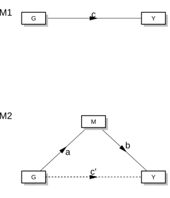
causal model (Figure 2.1).
In a mediation model (Figure 2.1), an independent variableX is assumed to cause a
set of mediatorsM, which, in turn, causes the dependent variable Y, so that the effect
of X on Y is at least partially through the effect of the mediators. The easiest case
of mediation models is the situation when there is only a single mediator M, the effect
of which can be modeled through linear regression (Figure 2.1 Panel A & B). In 1986,
Baron and Kenny (6) presented a pioneer yet simple mediation model, called causal
Figure 2.1: Mediation Diagram
causal relationship if the following four steps are satisfied:
1) the independent variable X is correlated with the outcome Y.
Y =α1+cX +ε1 (2.18)
2) X is correlated with potential mediator M
M =α2+aX+ε2 (2.19)
3) M is associated with the outcome variableY conditional on X
Y =α3 +c0X+bM +ε3 (2.20)
4) To establish that M completely mediate the relationship between X and Y, the
residual effect of X onY should be zero after controlling for M (path c0 Figure 2.1
The original Baron and Kenny approach did not include additional covariates in
the model to adjust for confounding effect. Further studies allowed confounding effect
to be corrected by adding extra covariates in the linear models. In this review, we
will present the models without considering additional covariates, however, it should
be noted that cases with additional covariates is analogous to what is presented.
The first three steps were proposed to be tested through the ordinary least square
(OLS) regression models, with the fourth step only required for conclusion of complete
mediation, which can be assessed through a bootstrap approach (86). Other methods of
estimation, such as logistic regression, multilevel modeling, and structural equal model
were proposed in later studies to work with data with non-Gaussian distribution.
How-ever, the necessary steps are the same regardless of the analytic methods (58). More
contemporary researchers believe that only step 2 and 3 are essential in establishing
mediation, especially in the situation of inconsistent mediations (87). Although
alterna-tive models have been proposed, causal steps models still constitute a large proportion
of all mediation tests in psychology and epidemiology studies (123, 168).
The amount of mediation is considered as indirect effect. From equations (2.18),(2.19)
and (2.20),
c=c0+ab (2.21)
wherecis the total effect of X onY,c0 is the direct effect andabis the indirect effect.
Equation (2.21) holds exactly when a) OLS was used in each of the steps, b) the
same cases are used in all analysis and c) all equations adjust for the same covariates.
The decomposition of the total effect into direct effect and indirect effect provides
the philosophical foundation that can be generalized to more complex causal inference
models, including structure equation models and models with counterfactual effects
There are several ways to test for the indirect effect under the causal steps
frame-work. A first and intuitive way to test for the null hypothesis of indirect effect ab= 0
is to test that both paths a and b are zero. A more highly recommended strategy to
test for the indirect effectab is to have a single test of ab (125). Sobel (191) proposed
a method that uses the asymptotical normal distribution of ab and corresponding Z
statistic to calculate p-values via Delta method. The approximate standard error of ab
is b2s2a+a2sb2 where sa and sb are the standard errors of a and b. The Sobel test is
considered to be very conservative and usually have low power (127) because the test
approximates ab by a symmetric normal distribution while the sample distribution is
usually highly skewed.
Bootstrapping method is a relatively new and increasingly popular approach in
test-ing the indirect effect (186, 16), which computes the nonsymmetric confidence bounds
for ab from the empirical distribution by resampling approach. There are two
com-monly used Bootstrap methods in literature. Percentile Bootstrap directly construct
the empirical distribution and confidence interval by finding the corresponding
per-centiles from the estimates from resampled data sets. Bias corrected Bootstrap
meth-ods (126, 93) calculate confidence interval and p-values by adjusting the bias between
the bootstrapped distribution and the indirect effect. Several recent studies have raised
concerns that the bias corrected bootstrapping test can have type I error that are too
liberal. In a recent paper (70), Hayes and Scharkow recommended using the bias
cor-rected bootstrap if the power is the main concern while use the percentile bootstrap
when the major concern is type I error.
In the cases when outcomeY are categorical variables, the OLS regression approach
is no longer applicable. However, the conceptual decomposition of the total effect into
use the modified models for estimation of the standard errors ofab:
Y0∗ =α1+cX+δ1 (2.22)
and
Y0∗ =α1+c0X+bM +δ2 (2.23)
where Y0∗ is the the unobserved probit of the probability of being in one of the two
categories of the outcome variable,c reflects the effect of the program on the probit of
the outcome probability in the first equation, c0 is the direct effect of the program on
the probit of outcome probability adjusted for the effects of the mediator,δ1 and δ2 are
the residuals in the probit models. The same Sobel tests and Bootstrap approach can
be used to test for the indirect effect.
Mediation with Multiple Mediators
Scientific and social researches are replete with situations when multiple
media-tors exist between an independent variable X and an outcome variable Y. Multiple
mediation models that incorporate simultaneous mediation by multiple variables have
received less attention in methodological and applied studies than the single mediation
models. However, there are a considerable number of methods proposed that aim to
test for the overall effect of multiple mediation (192, 19, 31, 124, 93).
Figure 2.1 Panel C represents the situation in which there are j possible mediators
between independent variableX and outcomeY. A specific indirect effect through one
mediator can be defined as the product of the two paths linking X to Y via one of
the mediators (19) and the total indirect effect are defined as the summation of all the
specific indirect effectPj
i=1aibi wherei= 1, ..., j. Similar to the single mediation case,
the total effect can be written asc=c0+Pj
and Hayes (93) emphasized the difference between the indirect effect through one of the
mediators (e.g.,M1) in a multiple mediation model and the indirect effect in a single
mediation model with only M1 as a mediator. They proposed three testing approaches
for the total indirect effect Pj
i=1aibi that mimic the three testing approaches in single
mediation analysis: 1) the causal steps approach, which tests for each specific indirect
effect and concludes mediation if any of the indirect effect is not zero. 2)
Product-of-Coefficients approach which derives the asymptotical variance of the total indirect
effectPj
i=1aibi using multivariate delta method and calculates p-values and confidence
interval through the usual Z test. Similar as the Soblel test, this method relies on
large sample approximation and can result in a lower power if the sample size and/or
effect size are not sufficiently large. 3) Bootstrapping approach, which uses resampling
procedure to establish the empirical distribution of the total indirect effect. Preacher
and Hayes (93) recommended the use to biased corrected Bootstrapping method for
testing of multiple mediation effect.
2.4.2 Counterfactual Approach to Mediation Analysis
While the concept of mediation, defined as indirect effect through the classical
regression framework, is appealing theoretically, it is difficult to extend this definition
to situations when the effect of exposure and mediator on the outcome have interactions
or is non-linear (164, 153). The approach of decomposing the total effect to direct and
indirect effect is not readily applicable because holding the mediator at different levels
would generate different direct effect at the presence of interaction effect.
Recent progress in mediation analysis has extended the concept of direct and
indi-rect effect to situations when non-linearities and interactions are present and considers
the identifiability conditions for a causal relationship. In a paper in 2001, Pearl et
effect: the controlled direct effect (CDE) and natural direct effect (NDE). Under the
counterfactual framework, the CDE of the exposure on the outcome is defined as
E(Y(x, m)−Y(x∗, m)|C), which is the change in the outcome if the treatment was changed from x∗ = 0 to x = 1 while the mediator M is fixed at level m across the
population, where C is the confounders that need to be adjusted for. The NDE is
defined asE(Y(x, M(x∗))−Y(x∗, M(x∗))), which is the exposure effect that would be obtained in the outcome if the exposure were changed from xtox∗ while the mediator
was kept at the level that would be observed as if the independent variable were kept
at x∗. Natural and controlled indirect effects (NID and CID) are defined as the
dif-ference between the total effect and the corresponding direct effect. VanderWeele and
Vansteelandt (209, 211) show that the counterfactual framework can extend the Baron
and Kenny formulae for direct and indirect effect to situations when there is interaction
effect between the exposure and mediator on the outcome.
Specifically, consider a model when there is interactive effect between the exposure
and mediator on the outcome,
E(M|X =x, C =c) =β0+β1x+β20c (2.24)
E(Y|X =x, M =m, C =c) =θ0+θ1x+θ2m+θ3xm+θ04c (2.25)
Through models (2.24) and (2.25), under some identifiability assumptions, the CDE,
NDE and NIE for change of independent variable from level x∗ to X is given by under
some identification assumptions
CDE = (θ1+θ3m)(x−x∗)
N DE = (θ1+θ3β0+θ3β1x∗+θ3β20c)(x−x∗)
N IE = (θ2β1+θ3β2a)(x−x∗)
In cases when there is no interaction effect (θ3 = 0), the CDE and NDE equal to the
direct effect obtained through the Baron-Kenny linear regression approach. However,
in this counterfactual framework, the total effect can be decomposed into the sum of
natural direct and indirect effect even in models with interactions and non-linearities
(153). NDE and NID are useful in evaluating the different mechanism of exposure on
outcome, while CDE and CID are often of greater interest in policy evaluation.
Certain identification assumptions are required for expression (2.26) to hold. The
direct and indirect effect defined previously are conditional on the levels of covariates C.
LetC = (C1, C2) where C1 denotes the confounders of the effect between the exposure
and outcome and C2 denotes the confounders of the mediator-outcome effect.
Accord-ing to VanderWeele et al.(209), two assumptions are required for the identifiability of
the controlled direct effect: 1) no unmeasured confounders of the exposure-outcome
relationship and 2) no unmeasured confounders of the mediator-outcome relationship.
Randomization in the treatment/exposure guarantees the first assumption, but not the
second assumption. Thus, in practice, it is required to control for the common causes of
treatment/exposure and the outcome to control for the first assumption and control for
common causes for mediators and the outcome for the second assumption. For the
iden-tification of natural direct and indirect effect, two additional assumptions are required:
3) no unmeasured confounders of the exposure-mediator effect, which will be
automati-cally satisfied if the treatment are randomized and 4) no unmeasured mediator-outcome
confounders affected by treatment. It is important to note that randomization can only
rule out the confounders with exposure effect but can not rule out confounding effect
2.4.3 Mediation Analysis in Genetic Analysis
Recently, mediation analysis has gained increasing interest in genetic studies to
dissect the direct and indirect effect of genetic variants on complex diseases (13, 66,
80, 216, 210, 46, 200, 140, 109, 174). Most of these studies used data from GWAS and
applied mediation methods that were developed through social science literatures or
epidemiological studies, typically with an assumption that the genomic variation such as
SNP, or a quantitative trait locus(QTL), acts as a causal anchor from which all arrows
in the corresponding causality diagram are directed outward. However reasonable this
assumption appears, cautions should be taken when the sampling scheme is not random,
such as in case control studies (104).
Up to now, most of these genetic studies involve analyzing the SNP-trait-trait triads,
in which only a single mediator is concerned. For example, Wang et al. used the
So-bel’s test for binary outcomes to evaluate the mediation effect of smoking and Chronic
Obstructive Pulmonary Disease (COPD) on the relations between CHRNA5-A3
ge-netic locus and lung cancer risk (216), with adjustment for age and other covariates.
Chen et al. (29) developed theoretical justification in the form of “causality
equiva-lence theorem”, stating the sufficient conditions required for a causal conclusion of the
SNP-trait-trait triads. This method has been used, with certain modifications, in
sev-eral rigorous yet conservative approaches to dissect genetic causal relationship between
genotypes and phenotypes, with gene expression or methylation as potential mediators
(140, 115).
Multiple mediation models have been explored in genetic studies as well.
Vander-Weele et al. (210) modeled smoking as a potential mediator between genetic variant
on 15q25.1 and lung cancer, while allowing for interaction effect between smoking and
COPD, in which mediation through smoking can account for only a small proportion
smoking and COPD constitute two steps in the causal pathway between
CHRNA5-A3 variant and lung cancer. Bootstrapping was used to assess the significance of the
CHAPTER 3
Global Analysis of Methylation via a Functional Regression Approach
3.1 Introduction
Recent advances in high-throughput biotechnology have culminated in the
devel-opment of large scale epigenome wide association studies (EWAS) (159) in which the
DNA methylation at hundreds of thousands of CpGs along the genome can be
simul-taneously measured across a large number of samples (10, 172). EWAS have resulted
in the identification of differentially methylated CpGs associated with differences in
disease states, clinical outcomes, environmental exposures, or other experimental
con-ditions (85, 184, 73, 74). These discoveries can provide a breadth of information from
fundamental insights into the mechanisms underlying complex disease and to potential
biomarkers for diagnosis or prognosis (98, 4).
Despite many successes, analysis of EWAS remains challenging (14). In addition to
open questions concerning preprocessing and normalization (44, 203, 132, 201),
associ-ation analysis with outcome variables is also difficult. Standard analysis proceeds via
individual CpG analysis wherein the association between each CpG and an outcome
variable (e.g. disease state, environmental exposure, etc.) is assessed one-by-one. After
computing a p-value for each CpG, multiple testing criteria such as the false discovery