www.atmos-chem-phys.net/16/9533/2016/ doi:10.5194/acp-16-9533-2016
© Author(s) 2016. CC Attribution 3.0 License.
Co-benefits of global and regional greenhouse gas mitigation
for US air quality in 2050
Yuqiang Zhang1, Jared H. Bowden1, Zachariah Adelman1,2, Vaishali Naik3, Larry W. Horowitz4, Steven J. Smith5, and J. Jason West1
1Environmental Sciences and Engineering Department, University of North Carolina at Chapel Hill,
Chapel Hill, NC 27599, USA
2Institute for the Environment, University of North Carolina at Chapel Hill, Chapel Hill, NC 27599, USA 3UCAR/NOAA Geophysical Fluid Dynamics Laboratory, Princeton, NJ 08540, USA
4NOAA Geophysical Fluid Dynamics Laboratory, Princeton, NJ 08540, USA
5Joint Global Change Research Institute, Pacific Northwest National Laboratory, College Park, MD 20740, USA
Correspondence to:J. Jason West ([email protected])
Received: 27 December 2015 – Published in Atmos. Chem. Phys. Discuss.: 21 January 2016 Revised: 13 June 2016 – Accepted: 2 July 2016 – Published: 1 August 2016
Abstract.Policies to mitigate greenhouse gas (GHG) emis-sions will not only slow climate change but can also have ancillary benefits of improved air quality. Here we examine the co-benefits of both global and regional GHG mitigation for US air quality in 2050 at fine resolution, using dynami-cal downsdynami-caling methods, building on a previous global co-benefits study (West et al., 2013). The co-co-benefits for US air quality are quantified via two mechanisms: through re-ductions in co-emitted air pollutants from the same sources and by slowing climate change and its influence on air qual-ity, following West et al. (2013). Additionally, we separate the total co-benefits into contributions from domestic GHG mitigation vs. mitigation in foreign countries. We use the Weather Research and Forecasting (WRF) model to dynam-ically downscale future global climate to the regional scale and the Sparse Matrix Operator Kernel Emissions (SMOKE) program to directly process global anthropogenic emissions to the regional domain, and we provide dynamical bound-ary conditions from global simulations to the regional Com-munity Multi-scale Air Quality (CMAQ) model. The total co-benefits of global GHG mitigation from the RCP4.5 sce-nario compared with its reference are estimated to be higher in the eastern US (ranging from 0.6 to 1.0 µg m−3) than
the west (0–0.4 µg m−3)for fine particulate matter (PM2.5),
with an average of 0.47 µg m−3over the US; for O3, the
to-tal co-benefits are more uniform at 2–5 ppb, with a US av-erage of 3.55 ppb. Comparing the two mechanisms of
co-benefits, we find that reductions in co-emitted air pollutants have a much greater influence on both PM2.5 (96 % of the
total co-benefits) and O3(89 % of the total) than the second
co-benefits mechanism via slowing climate change, consis-tent with West et al. (2013). GHG mitigation from foreign countries contributes more to the US O3 reduction (76 %
of the total) than that from domestic GHG mitigation only (24 %), highlighting the importance of global methane re-ductions and the intercontinental transport of air pollutants. For PM2.5, the benefits of domestic GHG control are greater
(74 % of total). Since foreign contributions to co-benefits can be substantial, with foreign O3 benefits much larger than
those from domestic reductions, previous studies that focus on local or regional co-benefits may greatly underestimate the total co-benefits of global GHG reductions. We conclude that the US can gain significantly greater domestic air quality co-benefits by engaging with other nations to control GHGs.
1 Introduction
emissions (biogenic gases and particles, dust, fire and light-ing) that influence air quality. Second, air pollutants such as particulate matter (PM) and ozone (O3) can change the
climate by altering the solar and terrestrial radiation bal-ance through direct and indirect effects (Myhre et al., 2013). Third, the sources of emissions of greenhouse gases (GHGs) and air pollutants are usually shared, particularly through the combustion of fossil fuels, so actions to control one can also influence emissions of the other. Policies to control GHG emissions will therefore not only slow climate change in the future but will also provide co-benefits of improvements to air quality and consequently to human health (Bell et al., 2008; Nemet et al., 2010).
Recent studies that model future air quality have focused on the effects of single or combined changes in future cli-mate and emissions on global and regional air quality, using both global and regional chemical transport models (CTMs; Weaver et al., 2009; Jacob and Winner, 2009; Fiore et al., 2012). Climate change is likely to decrease background O3
over remote places due to the elevated humidity and increase O3over urban and polluted areas, in part because of higher
temperature. Jacob and Winner (2009) concluded that future climate change could increase summertime O3by 1–10 ppb
over polluted regions in the US in scenarios from the Spe-cial Report on Emission Scenarios (SRES; Nakicenovic and Swart, 2000). In one study, climate change in 2050 under the SRES A1B scenario is projected to increase summertime O3by 2–5 ppb over large areas in the US, comparable to the
effect of reduced anthropogenic emissions of O3precursors
which reduces O3by 2–15 ppb, especially in the east (Wu et
al., 2008). The overall effect of climate change on PM is less clear, as different components of PM may respond differently to changes in climate variables (Jacob and Winner, 2009; Tai et al., 2010; Fiore et al., 2012, 2015).
Many studies have also estimated the co-benefits of re-gional or local GHG mitigation for air quality and human health through reductions in co-emitted air pollutants. Ci-fuentes et al. (2001) found that GHG mitigation through re-duced fossil fuel combustion could bring significant local air-pollution-related health benefits to some megacities. These health benefits have been estimated in many studies (Bell et al., 2008) and give co-benefits ranging from $2–196 t CO−21 when monetized, comparable to the costs of GHG reduc-tions (Nemet et al., 2010). A few studies also analyze the co-benefits for future air quality and human health from future regional GHG mitigation scenarios (Thompson et al., 2014; Trail et al., 2015). Thompson et al. (2014) studied the co-benefits of different US climate policies for 2030 domestic air quality and found that when monetized, the human health benefits due to the improved air quality can offset 26–1050 % of the cost of the carbon polices, depending on the policy.
These benefit studies may underestimate the total co-benefits as they only consider local or regional climate poli-cies, neglecting benefits outside of the region considered and benefits within those regions from global GHG
mitiga-tion. The total co-benefits of global mitigation are relevant as meaningful GHG mitigation requires participation from at least several of the most highly emitting nations. We exam-ined the co-benefits of global GHG reductions for both global and regional air quality and human health, using a global atmospheric model (Model for OZone And Related chemi-cal Tracers, version 4, MOZART-4, hereafter referred to as MZ4) and self-consistent future scenarios (West et al., 2013, referenced hereafter as WEST2013). In addition to evaluat-ing co-benefits through reductions in co-emitted air pollu-tants, WEST2013 was the first study to quantify co-benefits through a second mechanism: slowing climate change and its effects on air quality. There are several other innovations of WEST2013: we account for global air pollution transport and long-term influences of methane using the global CTM; we consider realistic scenarios in which air pollutant emis-sions, demographics and economic valuation are modeled consistently; and we evaluate chronic mortality influences of fine PM (PM2.5, PM with diameter smaller than 2.5 µm)
as well as O3. WEST2013 concluded that global GHG
mit-igation could bring significant air quality improvement for both PM2.5 and O3 and avoid 2.2±0.8 million premature
deaths globally by 2100 due to the improved air quality. When monetized, the global average marginal co-benefits of avoided mortality were $50–380 t CO−21, higher than the pre-vious estimates (Nemet et al., 2010). The co-benefits from the first mechanism of reduced co-emitted air pollutants were shown to be much greater than the co-benefits from the sec-ond mechanism via slowing climate change.
The WEST2013 study is limited by the coarse resolution of the CTM used (2◦×2.5◦ horizontally). Here we inves-tigate the co-benefits of global GHG mitigation for US air quality at much finer resolution (36 km×36 km), building on the scenarios in the global study. WEST2013 simulated co-benefits in 2030, 2050 and 2100, and we choose here to downscale the results in 2050, as climate change influences air quality by 2050, and it is within the time frame of cur-rent decision making for both climate change and air quality. We use a comprehensive modeling framework in the down-scaling process, including a regional climate model to dy-namically downscale the global climate to the contiguous United States (CONUS), an emissions processing program to directly process the global anthropogenic emissions to the regional scale, and we create dynamical boundary conditions (BCs) from the global co-benefit outputs for the regional CTM. We quantify the total co-benefits of global GHG miti-gation for US air quality for both PM2.5and O3and then
sep-arate the co-benefits from the two mechanisms analyzed by WEST2013. We also quantify the co-benefits from domes-tic GHG mitigation vs. the co-benefits from those of foreign countries’ reductions. We then present the co-benefits from global and domestic GHG mitigation for nine US regions.
co-benefit of slowing climate change from GHG mitigation and by analyzing that co-benefit through realistic future sce-narios, following WEST2013. With regard to previous co-benefits studies that have been conducted on a regional scale (e.g., Thompson et al., 2014), this research differs by em-bedding the regional co-benefits study in a consistent global context, accounting for the effects of changes in global air pollutant emissions and climate change on US air quality.
2 Methodology
Future air quality changes under global and regional GHG mitigation scenarios are simulated using a regional CTM. The scenarios modeled here are built on those of WEST2013, who compared the Representative Concentration Pathway 4.5 (RCP4.5) scenario with its associated reference scenario (REF). Air pollutant emissions in REF are state-of-the-art long-term emissions projections created by using the Global Change Assessment Model (GCAM; Thomson et al., 2011). RCP4.5 was developed based on REF by applying a global carbon price to all world regions and all sectors including carbon in terrestrial systems. As discussed by van Vuuren et al. (2011), the air pollutant emissions for the four RCP scenarios were prepared by different groups using different models and assumptions, so they are inconsistent with one another. But by comparing REF with RCP4.5, we use a self-consistent pair of scenarios, where the difference is uniquely attributed to a climate policy. WEST2013 used both emis-sions and meteorology from RCP4.5 to simulate future air quality under the RCP4.5 climate policy and used emissions from REF and meteorology from RCP8.5 to simulate future air quality assuming no climate policy. Since no general cir-culation model (GCM) conducted future climate simulations for the REF scenario, RCP8.5 is used as a proxy for the fu-ture climate under REF. The differences between these two scenarios give the total co-benefits for future air quality un-der climate policy from RCP4.5. Through one extra simula-tion with emissions from RCP4.5 together with RCP8.5 me-teorology (e45m85 in Table 1) and by comparing with REF and RCP4.5, WEST2013 separated the total co-benefits into the two mechanisms: the benefits from reductions in co-emitted air pollutants and co-benefits from slowing climate change and its influence on air quality.
Here we conduct downscaling processes to provide fine-resolution inputs for the regional CTM. We use the Weather Research and Forecasting model version 3.4.1 (WRF; Ska-marock and Klemp, 2008) to downscale the future global cli-mate from the GCM to the regional scale at a horizontal res-olution of 36×36 km for the CONUS. We directly process global anthropogenic emissions to regional scale using the Sparse Matrix Operator Kernel Emissions (SMOKE, v3.5, Houyoux et al., 2000) program. The outputs from the global MZ4 simulations of WEST2013 (Table 1) are downscaled to provide initial conditions (ICs) and dynamic hourly BCs
for the regional CTM. The latest version of the Community Multi-scale Air Quality model (CMAQ, v5.0.1; Byun and Schere, 2006) is used as the regional CTM to simulate air quality changes over the CONUS domain. WEST2013 simu-lated 5 consecutive years for each scenario and used the last 4 years’ average for the data analysis with the first year as a spin-up. Due to the limitations of computational resources, we run CMAQ for 40 months consecutively for each sce-nario, with the first 4 months as spin-up, and analyze the re-sults as 3-year averages.
2.1 Regional meteorology
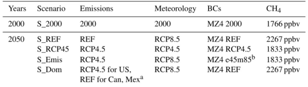
Table 1.List of CMAQv5.0.1 simulations in this study. Hourly BCs are from the MOZART-4 (MZ4) simulations of WEST2013. We fix the methane (CH4)background concentrations in CMAQ consistent with the RCP scenarios and WEST2013.
Years Scenario Emissions Meteorology BCs CH4
2000 S_2000 2000 2000 MZ4 2000 1766 ppbv
2050 S_REF REF RCP8.5 MZ4 REF 2267 ppbv
S_RCP45 RCP4.5 RCP4.5 MZ4 RCP4.5 1833 ppbv
S_Emis RCP4.5 RCP8.5 MZ4 e45m85b 1833 ppbv
S_Dom RCP4.5 for US, RCP8.5 MZ4 REF 2267 ppbv
REF for Can, Mexa
aThe part of Canada and Mexico in the domain.bGlobal simulation using RCP4.5 emissions together with RCP8.5
meteorology in 2050.
Figure 1.Changes in(a)2 m temperature (◦C) and(b)precipitation (mm day−1)centered on 2050 between RCP8.5 and RCP4.5 (RCP8.5–
RCP4.5).
We compare the downscaled WRF and the global GFDL AM3 simulations (for 3-year averages instead of 4 to be consistent with CMAQ outputs below), for 2 m tempera-ture (T2) with 21 years (1979 to 2000) of observation data from the 32 km North America Regional Reanalysis (NARR; Mesinger et al., 2006) and for precipitation with 41 years (1948 to 1998) of observation data from the 0.25◦×0.25◦ Unified US precipitation data product from the NOAA Cli-mate Prediction Center (Higgins et al., 2000). The large-scale spatial patterns for both T2 and precipitation between WRF and GFDL AM3 are similar (Fig. S1 in the Supplement). However, the downscaled simulations help resolve impor-tant features that influence the average regional climate, such as those related to topography. Comparing WRF future pro-jected change centered on 2050 with 2000, we see that the 3-year average of T2 generally increases over the entire US for both RCP8.5 and RCP4.5 (Figs. S2–S3). Temperature increases are largest for extreme northeastern latitudes, the southeast and southwest US in both scenarios, with a US av-erage warming of 3.05 and 2.59◦C for RCP8.5 and RCP4.5, respectively. Additionally, precipitation is projected to
de-crease over most of the US in both scenarios with a US av-erage decrease of 0.20 and 0.15 mm day−1 in RCP8.5 and RCP4.5. Comparing the changes between scenarios (RCP8.5 minus RCP4.5), Fig. 1 illustrates that temperature increases are smaller in RCP4.5 throughout the CONUS, except in the northwest. The precipitation difference between scenarios has a larger spatial variability than the T2. Ignoring other in-fluences of climate change, decreases in precipitation would be expected to decrease PM wet scavenging and increase PM concentration.
2.2 Regional emissions
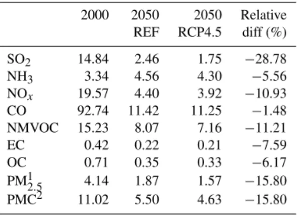
Table 2.Anthropogenic emissions in the US for major air pollutants in 2000 and 2050 from REF and RCP4.5 (Tg yr−1)and the rela-tive differences (Relarela-tive diff) between RCP4.5 and REF in 2050 ((RCP4.5 – REF)/REF×100).
2000 2050 2050 Relative REF RCP4.5 diff (%)
SO2 14.84 2.46 1.75 −28.78
NH3 3.34 4.56 4.30 −5.56
NOx 19.57 4.40 3.92 −10.93
CO 92.74 11.42 11.25 −1.48
NMVOC 15.23 8.07 7.16 −11.21
EC 0.42 0.22 0.21 −7.59
OC 0.71 0.35 0.33 −6.17
PM12.5 4.14 1.87 1.57 −15.80 PMC2 11.02 5.50 4.63 −15.80
1,2PM
2.5and PMC are the total emissions back-calculated based
on the EC and OC.
global emissions in 2000 and in 2050 from REF and RCP4.5 to provide temporally and spatially resolved CMAQ emis-sion input files. We first regrid the global emisemis-sions datasets at 0.5◦×0.5◦with finer resolution (36 km×36 km) and then apply source-specific temporal and speciation profiles from the NEI to assign temporal variations and re-speciate the PM and volatile organic compound (VOC) species. By regridding the REF and RCP4.5 data, we account better for changes in the spatial distribution changes in future emissions pro-jected in the RCPs (Figs. S4–S10) but do not provide addi-tional spatial detail beyond what is provided by the RCPs at 0.5◦resolution, whereas the traditional method only consid-ers changes in the magnitude of air pollutants in the future, assuming a constant spatial and sectoral distribution. We use constant (year 2000) land use and land cover for all simula-tions in WRF and CMAQ, whereas the spatial distribusimula-tions of anthropogenic emissions change in the RCP scenarios.
In addition, the RCP datasets report only elemental carbon (EC) and organic carbon (OC) but ignore emissions of other primary PM species. Here we back-calculate the total PM2.5 and PM coarse (PMC) primary emissions for all
sectors from the reported EC and OC. We first derive the emission fractions of EC and OC in each sector by cross-comparing the definitions of the sectors in IPCC, the Source Clarification Codes (SCC) in the speciation cross-reference file (http://www.airqualitymodeling.org/cmaqwiki/index. php?title=CMAQv5.0_GSREF_example) and the NEI PM speciation profile file (http://www.airqualitymodeling.org/ cmaqwiki/index.php?titleCMAQv5.0_GSPRO_Example, Table S1 in the Supplement). In back-calculating total PM emissions from BC and OC, there is usually more than one subcategory within one sector; e.g., the sector “Industries” includes emissions from the subcategory of “1A2_2A_B_C_D_E” (Table S1). When that happens, we use the speciation cross-reference file from the subcategory
with the largest mass fraction in this sector, following the methods of Reff et al. (2009) and Xing et al. (2013). Then we calculate the total PM2.5 and PMC in each grid cell
by dividing the reported EC and OC by their emission fractions individually and average these two. By doing this, we increase the total PM2.5 emissions of the RCPs
by incorporating the inorganic components of primary PM, such as sulfate and nitrate. We check these results by comparing the total 2000 PM2.5 emissions of 4.14 Tg yr−1
in this study (Table 2) with other studies, finding that it is comparable to the total of 4.69 Tg yr−1in 2001 from the US NEI (http://www.epa.gov/ttnchie1/trends/). Our calculated PM2.5emission is also lower than the estimated 5.53 Tg yr−1
in 2000 by Xing et al. (2013), which used an activity data-based approach to develop consistent temporally resolved emissions from 1999 to 2010.
In Table 2, we list the US anthropogenic emissions for ma-jor air pollutants in 2000 and 2050 from REF and RCP4.5. Significant decreases are seen for most pollutants from 2000 to 2050 for both REF and RCP4.5, except for NH3 which
is projected to increase due to agricultural activity (van Vuuren et al., 2011). Comparing RCP4.5 and REF, emis-sions of PM2.5 and O3 precursors also decrease, including
EC (7.59 %) and OC (6.17 %), with NOx and non-methane
volatile organic compounds (NMVOCs) decreasing by more than 10 %. SO2 has the largest relative decreases between
RCP4.5 and REF in 2050 (28.78 %). Large spatial variations in emissions reductions are also seen over the US, with the largest reductions seen in the east and west urban areas of US for most air pollutants and smaller reductions in the Great Plains (Figs. S4–S10).
Biogenic emissions are estimated using the Biogenic Emission Inventory System (BEIS v3.14), which responds to the changing climate for different scenarios. It is config-ured to run online in CMAQ and calculates the emissions of 35 chemical species, including 14 monoterpenes and 1 sesquiterpene. We assume that land use and land cover will stay constant in the future for the purpose of estimating bio-genic emissions. We also use the BEIS online calculation for natural soil NOxemissions. The online option of lightning is
also turned on to calculate the NOxemissions by estimating
the number of lightning flashes based on the modeled con-vective precipitation, which also changes with climate. We prepare the ocean–land mask for the domain to calculate sea salt emissions, which can be significant in coastal environ-ments (Kelly et al., 2010).
2.3 Regional air quality model and dynamical chemical BCs
(Reff et al., 2009), oxidative aging of primary organic carbon (Simon and Bhave, 2012), and an updated treatment and tracking of crustal species (e.g., Ca2+, K+, Mg2+)and trace metals (e.g., Fe, Mn; Fountoukis and Nenes, 2007). Several other enhancements in v5.0 of CMAQ were discussed by Appel et al. (2013) and Nolte et al. (2015), and there are no significant changes for the aerosol module between v5.0 and v5.0.1 (http://www.airqualitymodeling.org/cmaqwiki/index. php?titleCMAQ_version_5.0.128July_2012_release29_ Technical_Documentation). The model is configured with 34 vertical layers, with the lowest level being 34 m high, to the highest level at 50 hPa. The horizontal resolution is 36 km by 36 km for the CONUS domain. PM2.5 is
calculated from the CMAQ output as the sum of the species EC, OC, secondary organic aerosol (SOA), non-carbon organic matter (NCOM), nitrate (NO−3), sulfate (SO24−), ammonium (NH+4), sodium (Na+), chloride (Cl−), eight crustal and trace metal species, and other unspeciated fine PM (OTHER).
The dynamical BCs for this study are provided by the global MZ4 simulations of WEST2013. The hourly bound-ary values from MZ4 are horizontally interpolated from coarser resolution to the regional finer resolution and also vertically interpolated as MZ4 and CMAQ have different vertical layers. Chemical species are mapped between MZ4 and CMAQ v5.0.1, due to the different chemical mechanisms used by these two models, following the descriptions of Em-mons et al. (2010) and ENVIRON (http://www.camx.com/ download/support-software.aspx). For the chemical species in CMAQ that do not exist in MZ4, values are set to defaults as suggested by the CMAQ website.
2.4 Scenarios
We simulate scenarios in CMAQ comparable to WEST2013, except that we carry out one extra scenario to quantify the co-benefits from domestic vs. foreign GHG mitigation (Table 1). S_2000 is conducted to evaluate CMAQ model performance and to compare it with future scenarios. For this study, we run four scenarios in 2050. The differences between S_RCP45 and S_REF are the total co-benefits for US air quality from global GHG mitigation. The emission benefit from the first mechanism is calculated as the difference between S_ Emis and S_REF, for which the change in methane concentra-tion is included as an emission benefit and the meteorol-ogy benefit is calculated as S_RCP45 minus S_Emis. By comparing S_Dom (applying GHG mitigation from RCP4.5 scenario in the US only) with S_REF and S_RCP45 with S_Dom, we quantify the co-benefits from domestic and for-eign GHG mitigation. The co-benefits from forfor-eign reduc-tions are found by simple subtraction (S_RCP45 – S_REF) – (S_Dom – S_REF)=S_RCP45 – S_Dom. In estimating the co-benefits of domestic reductions, we account for the influences of methane and of global climate change as for-eign influences (as most methane and GHG emissions are
outside of the US) and assume that US air pollutant emis-sions have small effects on global or regional climate, such as through aerosol forcing. In each scenario, we fix global methane at concentrations given by the RCPs (Table 1) and account for methane changes as a foreign influence, neglect-ing the fraction of global anthropogenic methane emissions that are from the US (7.4 % in 2050 REF scenario and 7.0 % in 2050 RCP4.5). All scenarios are set up as continuous runs, with S_2000 running from September 2000 to December 2003, with the first 4 months in 2000 as spin-up. The future scenarios are run from September 2049 to December 2052 with the months in 2049 as spin-up. Results are presented as the average of 3 years.
3 Results
3.1 CMAQ model evaluation
The CMAQ model has been broadly used to study regional future air quality (Hogrefe et al., 2004; Tagaris et al., 2007; Nolte et al., 2008; Lam et al., 2011; Gao et al., 2013) and has been evaluated in many applications (Appel et al., 2010, 2011, 2013; Nolte et al., 2015). Here we evaluate the CMAQ v5.0.1 performance by comparing the model outputs from S_2000 with observations in 2000 from the Interagency Monitoring of PROtected Visual Environments (IMPROVE; http://vista.cira.colostate.edu/improve/), the Chemical Spe-ciation Network (CSN; previously known as STN, http: //www.epa.gov/ttn/amtic/speciepg.html), the Clean Air Sta-tus and Trends Network (CASTNET; http://epa.gov/castnet/ javaweb/index.html) for total PM2.5 and its components,
and the EPA Air Quality System (AQS; http://www.epa.gov/ ttn/airs/airsaqs/detaildata/downloadaqsdata.htm) for O3. We
pair the model outputs with observations in space and time and calculate four groups of statistics to evaluate model per-formance: median bias (MdnB, µg m−3 for PM2.5 and ppb
for O3), normalized median bias (NMdnB, %), median
er-ror (MdnE, µg m−3 and ppb) and normalized median error (NMdnE, %, Supplement). Median metrics are used here in-stead of the mean, as for data with non-normal distributions (i.e., PM species) the median gives a better representation of the central tendency of the data (Appel et al., 2008). For O3evaluation, we use both the maximum daily 1 h (1 h_O3)
and maximum daily 8 h average (MDA8) and also calcu-late these metrics with a cutoff value of 40 ppb for the ob-served O3 to evaluate the model’s reliability in predicting
ozone values relevant for the national ambient air quality standards (NAAQS; USEPA, 2007). Model performance is not expected to be perfect as meteorology does not corre-spond with actual year 2000 meteorology and emissions are derived from global datasets rather than the specific NEI year dataset for the US
For total PM2.5, overall model performance is good and
Table 3.Evaluation of the S_2000 simulation (average of 3 years modeled) with surface observations in 2000 for PM2.5 (µg m−3)
and O3(ppb).
Pollutants MdnB NMdnB MdnE NMdnE
( %) ( %)
IMPROVE PM2.5 −0.89 −23.31 1.88 49.46 CSN PM2.5 −2.85 −27.44 4.29 41.30
AQS 1 h_O3 8.97 18.40 13.25 27.60
AQS 1 h_O3_40∗ 2.79 4.76 9.89 17.36
AQS MDA8_O3 11.87 28.01 14.13 33.35
AQS MDA8_O3_40∗ 3.95 7.37 9.09 16.95 *1 h_O
3_40 and MDA8_O3_40: observations below 40 ppb are excluded from the comparison.
slight differences in performance (Table 3). CMAQ under-estimates PM2.5 in these two networks and also its
compo-nents in all three networks (Table S2), except that it over-estimates SO24− compared with IMPROVE and NH+4 with CSN. Compared with other components, OC and EC are not well predicted, with higher NMdnB:−63.55 and−37.00 % in IMPROVE (OC and EC are not measured in the other two networks). In simulating PM2.5and its species, model
perfor-mance is better in winter than in summer (not shown here). The model overestimates surface O3as indicated by the
pos-itive MdnB (ppb) and NMdnB (%). The NMdnE for the 1 h O3 (MDA8-O3)declines from 27.60 (33.35 %) to 17.36 %
(16.95 %) after we apply the cutoff value of 40 ppb. The over-prediction is slightly lower for 1 h_O3 than for MDA8-O3;
however, this difference becomes smaller when we consider the cutoff values. By comparing the simulated annual PM2.5
and O3in 2000 (both are 3-year averages) between MZ4 and
CMAQ, we see that CMAQ captures urban-scale air quality better than MZ4 (Fig. S11).
3.2 Air quality changes in 2050
Here we show the seasonal and spatial patterns of future air quality changes centered in 2050 relative to 2000 from REF and RCP4.5 (Figs. S12 to S15). The 3-year seasonal aver-age of PM2.5 over the entire US decreases in 2050 in both
S_REF and S_RCP45 compared with S_2000, especially in the eastern US and California (CA). The seasonal decreases are largest in winter, with US averages in S_REF (S_RCP45) of 4.42 (4.88) µg m−3, and lowest in the summer of 1.55 (2.00) µg m−3, with annual average of 2.76 (3.23) µg m−3. The 3-year seasonal average of O3decrease significantly in
summer on both the east and west coast, with a US aver-age of 6.31 (9.50) ppb in S_REF (S_RCP45). O3increases
over the northeast and west US in winter in both S_REF and S_RCP45, caused by the weakened NO titration as a result of the large NO decrease in the two scenarios (Ta-ble 2), as also reported by other studies (Gao et al., 2013; Fiore et al., 2015), and the large methane increases in the RCP8.5 scenario (Gao et al., 2013). The magnitude of the decreases between S_REF and S_2000 is lower than that
&K DQ JH LQ 30 JP D & K DQ J H LQ R] R Q H S S E E –3
Figure 2. Comparison of annual US average concentration
changes for RCP4.5 in 2050 relative to 2000, for this study (black triangle), MZ4 from WEST2013 (red circle), and the ensemble mean (blue diamond) and multi-model range from ACCMIP (blue lines), for (a) PM2.5 and (b) O3. In panel (a),
the total PM2.5 reported by the ACCMIP models is shown on the left and the PM2.5 estimated as a sum of species
BC+OA+SOA+SO4+NO3+NH4+0.25×SeaSalt+0.1×Dust
following Fiore et al. (2012) and Silva et al. (2013) shown on the right. Values shown are the average of 3 years for CMAQ and MZ4 and 5 to 10 years for ACCMIP for three models (LMDzORINCA, GFDL-AM3 and GISS-E2-R) that report O3 and two models
(GFDL-AM3 and GISS-E2-R) that report PM2.5.
tween S_RCP45 and S_2000, as the REF scenario did not apply a GHG mitigation policy and thus has less emission reductions.
We then compare these air quality changes in 2050 with the MZ4 simulations of WEST2013 for both S_REF (Fig. S16) and S_RCP45 (Fig. 2) and for S_RCP45 with the ensemble model means from the Atmospheric Chemistry and Climate Model Intercomparison Project (ACCMIP; Lamar-que et al., 2013) following Fiore et al. (2012), as no AC-CMIP models simulated REF in 2050. For the US annual average PM2.5, the decrease in 2050 for S_RCP45 relative to
2000 in this study (3.23 µg m−3)is modestly higher than both the results from MZ4 and the ACCMIP ensemble mean but within the range of ACCMIP models when PM2.5 is
calcu-lated as a sum of species. The future O3changes in our study
(5.20 ppb) are clearly in the range of ACCMIP results and nearly identical to MZ4 (5.13 ppb). Comparisons of the air quality changes in 2050 for S_REF relative to 2000 between CMAQ and MZ4 are similar, except that the magnitudes of the changes are smaller than those for S_RCP45 (Fig. S16). CMAQ better simulates air quality changes in urban environ-ments on a finer scale compared with MZ4.
3.3 Total co-benefits for US air quality from global GHG mitigation
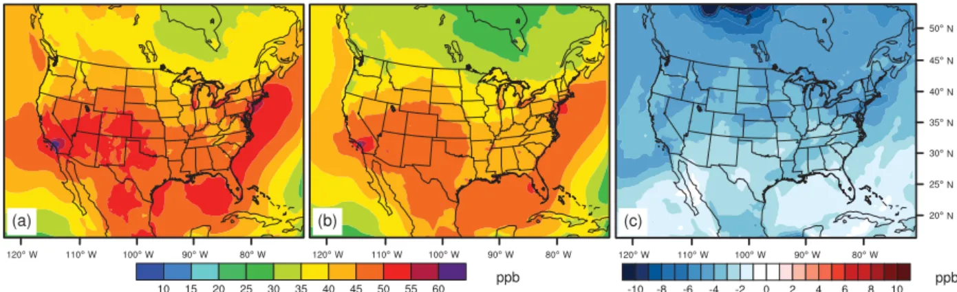
Projected 3-year average PM2.5 concentrations in 2050 in
(S_RCP45 minus S_REF) show notable decreases in major air pollutants in 2050. The total co-benefits for PM2.5 over
the US show a significant spatial gradient over the US do-main, which is greatest in the eastern US, especially urban ar-eas, as well as CA, ranging from 0.4 to 1.0 µg m−3, and least in the Rocky Mountains and northwest, with values below 0.4 µg m−3. The total co-benefits for PM2.5averaged over the
US are 0.47 µg m−3, with the largest contribution from or-ganic matter (OM, including primary OC, SOA and NCOM), accounting for 45 % of the total (0.21 µg m−3), followed by sulfate (0.11 µg m−3)and ammonia (0.05 µg m−3; Fig. S17). The total co-benefits are highest in fall, with a US domain average of 0.55 µg m−3, and lowest in spring (0.41 µg m−3; Fig. 4). Notice that the region with greatest co-benefits shifts from central areas in winter and spring to the east in summer and fall, with the largest component of OM also shifting from primary OC to SOA (Fig. S18).
Future O3 is presented here as the ozone season average
(from May to October) of MDA8. In general, 2050 O3
con-centrations in S_REF and S_RCP45 are projected to be high in the southern US, especially over the coastal areas and higher in the west than the east (Fig. 5). The total co-benefits for O3 are fairly uniformly significant over the entire US
domain, but slightly higher in the northeast and northwest and range from 2–5 ppb with a domain average of 3.55 ppb, unlike PM2.5, which is higher over urban regions. The
uni-formity of the total O3 co-benefits suggests that they are
strongly influenced by global O3reductions.
The total co-benefit for PM2.5 from this study
(0.47 µg m−3 over US) is lower than WEST2013 (area-weighted 3-year averages of 0.72 µg m−3 over the US), especially over the northwest and center of the US (Fig. S20). Analyzing the components of PM2.5, we find that
this difference is mainly caused by OM, with a US annual average of 0.40 µg m−3 in WEST2013 and 0.21 µg m−3 in this study (Fig. S21). For other components (EC, SO24−, NO−3 as reported in MZ4 of WEST2013), the CMAQ results are slightly lower than WEST2013 but share a similar spatial pattern (Figs. S22–S25). We expect that the total co-benefits of PM2.5in this study might be higher than WEST2013, as
we account for inorganic primary PM emissions in SMOKE. A possible explanation may be that different chemical mech-anisms and deposition processes are adopted for organic aerosols in MZ4 and CMAQ, which may lead to a shorter atmospheric lifetime for PM in CMAQ than in MZ4. The differences in the meteorology (e.g., the precipitation and temperature) between the downscaled WRF and the GFDL could also contribute to this difference. Total co-benefit of O3 from this study (3.55 ppb over US) is comparable to
WEST2013 (3.71 ppb) in both the magnitude and spatial distribution (Fig. S25).
3.4 Co-benefits from the two mechanisms
We quantify the co-benefits of global GHG mitigation for PM2.5and O3through two mechanisms: reduced co-emitted
air pollutants (S_Emis–S_REF) and slowing climate change and its effect on air quality (S_RCP45–S_Emis). The re-duction in co-emitted air pollutants has a much greater ef-fect than slowing climate change for PM2.5, accounting for
96 % of the US average PM2.5decrease. The emission
ben-efit for PM2.5over the US domain is 0.45 µg m−3and
great-est near urban areas where emissions are reduced (Fig. 6), with the largest contribution from OM (0.172 µg m−3 over the US), followed by sulfate (0.107 µg m−3)and ammonia (0.048 µg m−3). In Fig. S18, the OM decrease is caused
mainly by primary organic carbon (POC, 0.074 µg m−3
de-creases), followed by biogenic SOA (ORGB, 0.057 µg m−3)
and non-carbon organic matter (NCOM, 0.048 µg m−3). The POC and NCOM decreases are caused mainly by emission reductions, while the SOA decrease is caused mainly by changing climate (Fig. S19). Slowing climate change only accounts for 4 % of the US average total PM2.5 decreases
(0.02 µg m−3). It also has different signs of effect over the US, reducing PM2.5in the southern US but increasing in the
north.
For O3, the emission benefit is also larger than the climate
benefit, accounting for 89 % of the total O3 decreases
av-eraged over the US. The emission benefit for O3 over the
US domain is 3.16 ppb and much more uniform over the US, but slightly higher over the northeast and northwest. Slow-ing climate change accounts for 0.39 ppb O3 decreases –
11 % of the total and mainly in the Great Plains and the east, where temperatures are cooler under RCP4.5 compared with RCP8.5 (Fig. 1). The dominance of the emission co-benefit over the climate co-benefit for both PM2.5and O3is
consis-tent with WEST2013.
3.5 Co-benefits from domestic and foreign GHG mitigation
We also investigate the co-benefits from domestic GHG mit-igation by comparing S_Dom with S_REF, on the one hand, versus foreign GHG reductions by comparing S_RCP45 with S_Dom (Fig. 7), on the other hand. For PM2.5, domestic
GHG mitigation accounts for 74 % (0.35 µg m−3)of the to-tal PM2.5decrease over the whole US, with the greatest
ef-fect over the east and CA, where emissions of PM2.5and its
precursors are greatly reduced (Figs. S3–S9). The benefits from foreign GHG reductions for the US PM2.5change are
only obvious in the southern US, influenced by emission re-ductions in Mexico and global climate change. We conclude that domestic GHG mitigation has a greater influence on US PM2.5than reductions in foreign countries but that foreign
re-ductions also make a noticeable contribution, accounting for 26 % of total PM2.5decreases over the US and a greater
Figure 3.The 3-year average PM2.5(µg m−3)distributions in 2050 from(a)S_REF,(b)S_RCP45 and(c)the total co-benefits (shown as the difference between S_RCP45 and S_REF). Blue colors in panel(c)indicate an air quality improvement.
Figure 4.Seasonal distributions of total co-benefits for PM2.5(µg m−3)for(a)winter,(b)spring,(c)summer and(d)fall.
Note that the uncertainty in the foreign co-benefits is much larger than for the domestic reductions (Table S3). Longer simulations would be needed to reduce this uncertainty.
For O3, foreign countries’ GHG mitigation has a much
larger influence on the US, accounting for 76 % (2.69 ppb) of the total O3decrease, compared with 24 % from domestic
GHG mitigation (Fig. 7). The US experiences greater O3
de-creases in the north than the south, which is likely influenced in part by the air quality improvement in Western Canada as a result of slowing deforestation due to the climate policy in RCP4.5 (West et al., 2013). This large influence of for-eign reductions for O3 highlights the importance of global
methane reductions in RCP4.5 (anthropogenic emissions of 330 Tg yr−1in 2050 in RCP45, compared to 432 Tg yr−1in REF), particularly in Asia, and intercontinental transport.
3.6 Regional co-benefits and variability
We then quantify the co-benefits over nine US climate re-gions defined by the National Oceanic and Atmospheric Ad-ministration (Fig. S26) and their domestic and foreign com-ponents. The central, southeast, northeast and south regions have the largest total co-benefits for PM2.5(regional annual
north-Figure 5.The 3-year ozone season average (May to October) of MDA8 O3(ppb) from(a)S_REF,(b)S_RCP45 and(c)the total co-benefits
(shown as the difference between S_RCP45 and S_REF). Blue colors in panel(c)indicate an air quality improvement.
Figure 6.Benefits of reduced co-emitted air pollutants (a,b; S_Emis–S_REF) vs. slowing climate change (c,d; S_RCP45–S_Emis) for
PM2.5(a, c)and ozone season MDA8 surface O3(b, d). Blue colors indicate an air quality improvement. The numbers on the plots are the
3-year average of air quality changes over the US.
west has the lowest total co-benefits (0.16 µg m−3; Fig. 8).
Domestic GHG mitigation has the largest effect over these same regions and lowest effects over the northwest and west north central areas, with means of 0.13 µg m−3. Foreign co-benefits are greatest over the south, southwest, center and southeast and lowest over the northwest (Table S3). As a
Figure 7.Benefits of domestic (a,b; S_Dom–S_REF) vs. foreign(c, d)GHG reductions for PM2.5(a,c; S_RCP45–S_Dom) and ozone
season MDA8 surface O3(b, d). Blue colors indicate an air quality improvement. The numbers on the plots are the 3-year average of air
quality changes over the US.
For O3, the northeast, east north central and northwest
ar-eas have the highest total co-benefits (regional means of 4.61, 4.25 and 4.15 ppb; Fig. 9 and Table S3), although the total co-benefits for O3are fairly uniform over the US (Fig. 5). The
southeast has the lowest total co-benefits, with 2.67 ppb for the regional mean. Domestic co-benefits are higher over the center, northeast and southeast, with regional means of 1.25, 1.16 and 1.14 ppb, and lowest over the northwest (0.4 ppb). In general, foreign mitigation contributes more in the west than the east, most likely influenced by intercontinental transport from Asia. It is highest in the northwest, west north central and northeast areas, with regional means of 3.75, 3.45 and 3.45 ppb. The fraction of co-benefits from foreign mitigation is larger than 60 % in most regions, highest over the north-west (90 %) and lonorth-west over the southeast (57 %).
We also evaluate the variability in co-benefits for the 3 years simulated (Table S3). Over the US, the coefficient of variation (CV) for the total co-benefits for PM2.5 (7 %) is
much lower than that of the total co-benefits for O3(37 %),
which is controlled by the intercontinental transport and global CH4. The southeast has the highest CV (29 %) for
the total co-benefits of PM2.5, while other regions are lower
than 15 %, lowest in the east north central and northeast ar-eas (3 %). The southwest and south have the highest CV (70, 69 %) for the total co-benefits of O3 and the lowest in the
northwest (21 %). For regions with higher variability, longer simulations would be desirable to better quantify the annual average co-benefits.
4 Discussion
The co-benefits we present here are specific to the reference (REF) and mitigation (RCP4.5) scenarios we choose, and re-sults would differ for other baseline and mitigation scenarios. The estimated co-benefits also depend on the participation of many nations in the mitigation policies, and delaying partici-pation will likely change the co-benefits. However, we expect that the general features of these results are generalizable to other scenarios.
The total co-benefits for O3when downscaled are
fea-Figure 8.Mean values of domestic (blue) and foreign co-benefits (red) for US average(a)annual PM2.5and(b)ozone season MDA8
O3. The numbers below each bar are the percentage (%) of the
for-eign co-benefit.
tures better than the global model, such as the effects of to-pography and urban areas. For PM2.5, significant differences
are seen from the downscaling due to the fine resolution and different chemical mechanisms between the global and the regional model. The resolution we are using for this study (36 by 36 km) is fine enough for us to analyze the co-benefits at a state level but insufficient to fully resolve urban areas. Finer-resolution simulations (such as 12 by 12 km) with CMAQ or other CTMs can be carried out to better quantify the co-benefits over urban areas.
For this study, uncertainties and errors may exist under the assumptions and choices we make for each model. For ex-ample, uncertainties in the input meteorology and emissions data inventory have a significant influence on the CMAQ re-sults. Also, we see that the co-benefits of PM2.5 have large
contributions from OC and SOA over the central and east US (Figs. 4, S18). However, our model evaluations show that CMAQ greatly underestimates the total OC (primary OC and SOA) concentration compared with surface obser-vations. New gas-phase and aqueous-phase oxidation path-ways for SOA formation are found to play significant roles in producing organic aerosols (Lin et al., 2013; Pye and Pouliot, 2012; Pye et al., 2013), which are missing in the CMAQ version used in this study. We use the BEIS model to estimate the biogenic VOC (BVOC) emissions, but studies have shown that the BVOCs from the Model of Emissions
of Gases and Aerosols from Nature (MEGAN) are higher than those from BEIS by a factor of 2 (Pouliot, 2008; Pouliot and Pierce, 2009), which highlights the uncertainty in repre-senting these emissions and simulating both PM2.5 and O3
(Hogrefe et al., 2011).
We assume constant land use in the GCM, WRF and CMAQ when simulating the global and regional climate and estimating the biogenic emissions, which could introduce er-rors in our results (Unger, 2014; Heald and Spracklen, 2015). When we process the global anthropogenic emissions with SMOKE, we back-calculate the total PM2.5and PMC from
OC and BC, which introduces inorganic PM emissions and may make our results for co-benefits of PM2.5 higher. By
doing this, we account for missing emissions but also in-crease the total uncertainties in the emission inventory. Spec-tral nudging is adopted in this study to restrain WRF from drifting from the GCM, which has been shown to be bet-ter for some meteorological variables, but analysis nudging is better for others (Bowden et al., 2012, 2013; Otte et al., 2012). Moreover, only one model is used during downscaling for regional climate (WRF) and air quality (CMAQ) model-ing, and the mean of a model ensemble can be used to reduce model error. Simulations are based on 3-year averages, due to computational limitations, but these 3 years may reflect meteorological variability and not only climate change. This uncertainty may be greater for the total co-benefits of O3, for
which we see greater year-to-year variations than for PM2.5.
CMAQ simulations could be performed over more years to reduce the influence of the interannual climate variability. In separating domestic and foreign co-benefits, we assume that global and regional climate will be controlled by foreign GHG emissions and not influenced by GHG mitigation in the US, which introduces a small error into our results. We sim-ilarly attribute the global methane change to foreign influ-ence, as US methane emissions are a small fraction (6–10 %) of global emissions.
5 Conclusions
co-benefits from domestic GHG mitigation vs. foreign coun-tries’ reduction.
We find that there are significant benefits for both PM2.5
and O3over the US by 2050 from the global GHG
mitiga-tion in RCP4.5. The total co-benefits for PM2.5are higher in
the east than the west, with an average of 0.47 µg m−3over the US For O3, the total co-benefits are fairly uniform across
the US at 2–5 ppb, with a US average of 3.55 ppb. The co-benefits from reductions in co-emitted air pollutants have a greater influence on both PM2.5(accounting for 96 % of total
decreases) and O3(89 % of the total decreases) than the
sec-ond mechanism via slowing climate change, consistent with West et al. (2013).
Foreign countries’ GHG reductions have a much greater influence on the US O3reduction (76 % of the total)
com-pared with that from domestic GHG mitigation only (24 %), highlighting the importance of global methane reductions and the intercontinental transport of air pollutants. For PM2.5, the benefits of foreign GHG control are less than
domestic control but still a considerable portion of the to-tal (26 %). We conclude that the US can gain significantly greater domestic air quality co-benefits by engaging with other nations for GHG control to combat climate change, es-pecially for O3. This also applies to other nations which can
be expected to have ancillary air quality benefits from for-eign countries’ GHG mitigation. We also conclude that previ-ous studies that estimate co-benefits for one nation or region (e.g., Thomson et al., 2014), may significantly underestimate the full co-benefits when many countries reduce GHGs to-gether, particularly for O3.
6 Data availability
Inputs and outputs of all model simulations are archived at UNC’s mass storage system and can be obtained by contact-ing the correspondcontact-ing author.
The Supplement related to this article is available online at doi:10.5194/acp-16-9533-2016-supplement.
Acknowledgements. This publication was financially supported by the US Environmental Protection Agency (USEPA) STAR grant no. 834285 and the National Institute of Environmental Health Sciences grant no. 1 R21 ES022600-01. Its contents are solely the responsibility of the grantee and do not necessarily represent the official views of the USEPA or other funding sources. USEPA and other funding sources do not endorse the purchase of any commercial products or services mentioned in the publication.
Edited by: Q. Zhang
Reviewed by: two anonymous referees
References
Appel, K. W., Bhave, P. V., Gilliland, A. B., Sarwar, G., and Roselle, S. J.: Evaluation of the community multiscale air quality (CMAQ) model version 4.5: Sensitivities impacting model per-formance; Part II-particulate matter, Atmos. Environ., 42, 6057– 6066, doi:10.1016/j.atmosenv.2008.03.036, 2008.
Appel, K. W., Roselle, S. J., Gilliam, R. C., and Pleim, J. E.: Sensitivity of the Community Multiscale Air Quality (CMAQ) model v4.7 results for the eastern United States to MM5 and WRF meteorological drivers, Geosci. Model Dev., 3, 169–188, doi:10.5194/gmd-3-169-2010, 2010.
Appel, K. W., Foley, K. M., Bash, J. O., Pinder, R. W., Dennis, R. L., Allen, D. J., and Pickering, K.: A multi-resolution assessment of the Community Multiscale Air Quality (CMAQ) model v4.7 wet deposition estimates for 2002-2006, Geosci. Model Dev., 4, 357–371, doi:10.5194/gmd-4-357-2011, 2011.
Appel, K. W., Pouliot, G. A., Simon, H., Sarwar, G., Pye, H. O. T., Napelenok, S. L., Akhtar, F., and Roselle, S. J.: Evaluation of dust and trace metal estimates from the Community Multiscale Air Quality (CMAQ) model version 5.0, Geosci. Model Dev., 6, 883–899, doi:10.5194/gmd-6-883-2013, 2013.
Avise, J., Chen, J., Lamb, B., Wiedinmyer, C., Guenther, A., Salathé, E., and Mass, C.: Attribution of projected changes in summertime US ozone and PM2.5 concentrations to global
changes, Atmos. Chem. Phys., 9, 1111–1124, doi:10.5194/acp-9-1111-2009, 2009.
Bell, M. L., Davis, D. L., Cifuentes, L. A, Krupnick, A. J., Mor-genstern, R. D., and Thurston, G. D.: Ancillary human health benefits of improved air quality resulting from climate change mitigation, Environ. Health, 7, 41, doi:10.1186/1476-069X-7-41, 2008.
Bowden, J. H., Otte, T. L., Nolte, C. G., and Otte, M. J.: Examining Interior Grid Nudging Techniques Using Two-Way Nesting in the WRF Model for Regional Climate Modeling, J. Climate, 25, 2805–2823, doi:10.1175/JCLI-D-11-00167.1, 2012.
Bowden, J. H., Nolte, C. G., and Otte, T. L.: Simulating the impact of the large-scale circulation on the 2 m temperature and precipitation climatology, Clim. Dynam., 40, 1903–1920, doi:10.1007/s00382-012-1440-y, 2013.
Byun, D. and Schere, K. L.: Review of the Governing Equations, Computational Algorithms, and Other Compo-nents of the Models-3 Community Multiscale Air Quality (CMAQ) Modeling System, Appl. Mech. Rev., 59, 51–77, doi:10.1115/1.2128636, 2006.
Chen, F. and Dudhia, J.: Coupling an Advanced Land Surface– Hydrology Model with the Penn State–NCAR MM5 Model-ing System, Part I: Model Implementation and Sensitivity, Mon. Weather Rev., 129, 569–585, 2001.
Chen, J., Avise, J., Lamb, B., Salathé, E., Mass, C., Guenther, A., Wiedinmyer, C., Lamarque, J.-F., O’Neill, S., McKenzie, D., and Larkin, N.: The effects of global changes upon regional ozone pollution in the United States, Atmos. Chem. Phys., 9, 1125– 1141, doi:10.5194/acp-9-1125-2009, 2009.
Cifuentes, L., Borja-aburto, V. H., Gouveia, N., Thurston, G., and Davis, D. L.: Hidden Health Benefits of Greenhouse Gas Mitiga-tion, Science, 293, 1257–1259, 2001.
Freiden-reich, S. M., Gordon, C. T., Griffies, S. M., Held, I. M., Hurlin, W. J., Klein, S. A., Knutson, T. R., Langenhorst, A. R., Lee, H. C., Lin, Y., Magi, B. I., Malyshev, S. L., Milly, P. C. D., Naik, V., Nath, M. J., Pincus, R., Ploshay, J. J., Ramaswamy, V., Se-man, C. J., Shevliakova, E., Sirutis, J. J., Stern, W. F., Stouffer, R. J., Wilson, R. J., Winton, M., Wittenberg, A. T., and Zeng, F.: The dynamical core, physical parameterizations, and basic simu-lation characteristics of the atmospheric component AM3 of the GFDL global coupled model CM3, J. Climate, 24, 3484–3519, doi:10.1175/2011JCLI3955.1, 2011.
Emmons, L. K., Walters, S., Hess, P. G., Lamarque, J.-F., Pfister, G. G., Fillmore, D., Granier, C., Guenther, A., Kinnison, D., Laepple, T., Orlando, J., Tie, X., Tyndall, G., Wiedinmyer, C., Baughcum, S. L., and Kloster, S.: Description and evaluation of the Model for Ozone and Related chemical Tracers, version 4 (MOZART-4), Geosci. Model Dev., 3, 43–67, doi:10.5194/gmd-3-43-2010, 2010.
Fiore, A. M., Naik, V., Spracklen, D. V, Steiner, A., Unger, N., Prather, M., Bergmann, D., Cameron-Smith, P. J., Cionni, I., Collins, W. J., Dalsøren, S. , Eyring, V., Folberth, G. A, Ginoux, P., Horowitz, L. W., Josse, B., Lamarque, J.-F., MacKenzie, I. A, Nagashima, T., O’Connor, F. M., Righi, M., Rumbold, S. T., Shindell, D. T., Skeie, R. B., Sudo, K., Szopa, S., Takemura, T., and Zeng, G.: Global air quality and climate, Chem. Soc. Rev., 41, 6663–83, doi:10.1039/c2cs35095e, 2012.
Fiore, A. M., Naik, V., and Leibensperger, E. M.: Air Quality and Climate Connections, J. Air Waste Manage. Assoc., 65, 645–685, doi:10.1080/10962247.2015.1040526, 2015.
Fountoukis, C. and Nenes, A.: ISORROPIA II: a computa-tionally efficient thermodynamic equilibrium model for K+– Ca2+–Mg2+–NH+4–Na+–SO24−–NO−3–Cl−–H2O aerosols,
At-mos. Chem. Phys., 7, 4639–4659, doi:10.5194/acp-7-4639-2007, 2007.
Gao, Y., Fu, J. S., Drake, J. B., Lamarque, J.-F., and Liu, Y.: The impact of emission and climate change on ozone in the United States under representative concentration pathways (RCPs), At-mos. Chem. Phys., 13, 9607–9621, doi:10.5194/acp-13-9607-2013, 2013.
Grell, G. A. and Devenyi, D.: A generalized approach to parameterizing convection combining ensemble and data assimilation techniques, Geophys. Res. Lett., 29, 10–13, doi:10.1029/2002GL015311, 2002.
Heald, C. L. and Spracklen, D. V.: Land Use Change Impacts on Air Quality and Climate, Chem. Rev., 115, 4476–4496, doi:10.1021/cr500446g, 2015.
Higgins, R.W., Shi W., and Joyce, R.: Improved United States pre-cipitation quality control system and analysis, NCEP/Climate Prediction Center ATLAS No. 7, 2000.
Hogrefe, C., Lynn, B., Civerolo, K., Ku, J.-Y., Rosenthal, J., Rosen-zweig, C., Goldberg, R., Gaffin, S., Knowlton, K., and Kin-ney, P. L.: Simulating changes in regional air pollution over the eastern United States due to changes in global and re-gional climate and emissions, J. Geophys. Res., 109, D22301, doi:10.1029/2004JD004690, 2004.
Hogrefe, C., Isukapalli, S. S., Tang, X., Georgopoulos, P. G., He, S., Zalewsky, E. E., Hao, W., Ku, J.-Y., Key, T., and Sistla, G.: Impact of biogenic emission uncertainties on the simulated re-sponse of ozone and fine particulate matter to anthropogenic
emission reductions, J. Air Waste Manag. Assoc., 61, 92–108, doi:10.3155/1047-3289.61.1.92, 2011.
Hong, S. and Lim, J.: The WRF single-moment 6-class micro-physics scheme (WSM6), J. Korean Meteorol. Soc., 42, 129– 151, 2006.
Hong, S.-Y., Noh, Y., and Dudhia, J.: A New Vertical Diffusion Package with an Explicit Treatment of Entrainment Processes, Mon. Weather Rev., 134, 2318–2341, doi:10.1175/MWR3199.1, 2006.
Houyoux, M. R., Vukovich, J. M., Coats Jr., C. J., Wheeler, N. J. M., and Kasibhatla, P. S.: Emission inventory development and processing for the Seasonal Model for Regional Air Quality (SM-RAQ) project, J. Geophys. Res., 105, 9079–9090, 2000. Iacono, M. J., Delamere, J. S., Mlawer, E. J., Shephard, M.
W., Clough, S. A., and Collins, W. D.: Radiative forcing by long-lived greenhouse gases: Calculations with the AER ra-diative transfer models, J. Geophys. Res. Atmos., 113, 2–9, doi:10.1029/2008JD009944, 2008.
Jacob, D. J. and Winner, D. A.: Effect of climate change on air quality, Atmos. Environ., 43, 51–63, doi:10.1016/j.atmosenv.2008.09.051, 2009.
Kelly, J. T., Bhave, P. V., Nolte, C. G., Shankar, U., and Foley, K. M.: Simulating emission and chemical evolution of coarse sea-salt particles in the Community Multiscale Air Quality (CMAQ) model, Geosci. Model Dev., 3, 257–273, doi:10.5194/gmd-3-257-2010, 2010.
Lam, Y. F., Fu, J. S., Wu, S., and Mickley, L. J.: Impacts of fu-ture climate change and effects of biogenic emissions on surface ozone and particulate matter concentrations in the United States, Atmos. Chem. Phys., 11, 4789–4806, doi:10.5194/acp-11-4789-2011, 2011.
Lamarque, J.-F., Shindell, D. T., Josse, B., Young, P. J., Cionni, I., Eyring, V., Bergmann, D., Cameron-Smith, P., Collins, W. J., Do-herty, R., Dalsoren, S., Faluvegi, G., Folberth, G., Ghan, S. J., Horowitz, L. W., Lee, Y. H., MacKenzie, I. A., Nagashima, T., Naik, V., Plummer, D., Righi, M., Rumbold, S. T., Schulz, M., Skeie, R. B., Stevenson, D. S., Strode, S., Sudo, K., Szopa, S., Voulgarakis, A., and Zeng, G.: The Atmospheric Chemistry and Climate Model Intercomparison Project (ACCMIP): overview and description of models, simulations and climate diagnostics, Geosci. Model Dev., 6, 179–206, doi:10.5194/gmd-6-179-2013, 2013.
Lin, Y.-H., Zhang, H., Pye, H. O. T., Zhang, Z., Marth, W. J., Park, S., Arashiro, M., Cui, T., Budisulistiorini, S. H., Sexton, K. G., Vizuete, W., Xie, Y., Luecken, D. J., Piletic, I. R., Edney, E. O., Bartolotti, L. J., Gold, A., and Surratt, J. D.: Epoxide as a precur-sor to secondary organic aerosol formation from isoprene pho-tooxidation in the presence of nitrogen oxides., P. Natl. Acad. Sci. USA, 110, 6718–23, doi:10.1073/pnas.1221150110, 2013. Mesinger, F., DiMego, G., Kalnay, E., Mitchell, K., Shafran, P. C.,
Ebisuzaki, W., Jovic, D., Woollen, J., Rogers, E., Berbery ,E.H., Ek M. B., Fan, Y., Grumbine, R., Higgins, W., Li, H., Lin, Y., Manikin, G., Parrish, D., and Shi, W.: North American regional reanalysis, B. Am. Meteorol. Soc., 87, 343–360, 2006.
of Working Group I to the Fifth Assessment Report of the Inter-governmental Panel on Climate Change, edited by: Stocker, T. F., Qin, D., Plattner, G.-K., Tignor, M., Allen, S. K., Boschung, J., Nauels, A., Xia, Y., Bex, V., and Midgley, P. M., Cambridge Uni-versity Press, Cambridge, United Kingdom and New York, NY, USA, 659–740, doi:10.1017/CBO9781107415324.018, 2013. Naik, V., Horowitz, L. W., Fiore, A. M., Ginoux, P., Mao, J.,
Aghedo, A. M., and Levy, H.: Impact of preindustrial to present-day changes in short-lived pollutant emissions on atmospheric composition and climate forcing, J. Geophys. Res. Atmos., 118, 8086–8110, doi:10.1002/jgrd.50608, 2013.
Nakicenovic, N. and Swart, R.: Special Report on Emissions Sce-narios: A Special Report of Working Group III of the Inter-governmental Panel on Climate Change, Cambridge University Press, Cambridge, United Kingdom and New York, NY, USA, 2000.
Nemet, G. F., Holloway, T., and Meier, P.: Implications of in-corporating air-quality co-benefits into climate change poli-cymaking, Environ. Res. Lett., 5, 014007, doi:10.1088/1748-9326/5/1/014007, 2010.
Nolte, C. G., Gilliland, A. B., Hogrefe, C., and Mickley, L. J.: Link-ing global to regional models to assess future climate impacts on surface ozone levels in the United States, J. Geophys. Res., 113, D14307, doi:10.1029/2007JD008497, 2008.
Nolte, C. G., Appel, K. W., Kelly, J. T., Bhave, P. V., Fahey, K. M., Collett Jr., J. L., Zhang, L., and Young, J. O.: Evaluation of the Community Multiscale Air Quality (CMAQ) model v5.0 against size-resolved measurements of inorganic particle com-position across sites in North America, Geosci. Model Dev., 8, 2877–2892, doi:10.5194/gmd-8-2877-2015, 2015.
Otte, T. L. and Pleim, J. E.: The Meteorology-Chemistry Inter-face Processor (MCIP) for the CMAQ modeling system: up-dates through MCIPv3.4.1, Geosci. Model Dev., 3, 243–256, doi:10.5194/gmd-3-243-2010, 2010.
Otte, T. L., Nolte, C. G., Otte, M. J., and Bowden, J. H.: Does Nudg-ing Squelch the Extremes in Regional Climate ModelNudg-ing?, J. Cli-mate, 25, 7046–7066, doi:10.1175/JCLI-D-12-00048.1, 2012. Pouliot, G.: A Tale of Two Models: A Comparison of the Biogenic
Emission Inventory System (BEIS3.14) and Model of Emissions of Gases and Aerosols from Nature (MEGAN 2.04), 7th Annual CMAS Conference, Chapel Hill, NC, USA, 7 October 2008. Pouliot, G. and Pierce, T. E.: Integration of the Model of Emissions
of Gases and Aerosols from Nature (MEGAN) into the CMAQ Modeling System, 18th International Emission Inventory Con-ference, Baltimore, Maryland, 14–17 April 2009.
Pye, H. O. T. and Pouliot, G. A: Modeling the Role of Alkanes, Polycyclic Aromatic Hydrocarbons, and Their Oligomers in Sec-ondary Organic Aerosol Formation, Environ. Sci. Technol., 46, 6041–6047, doi:10.1021/es300409w, 2012.
Pye, H. O. T., Pinder, R. W., Piletic, I. R., Xie, Y., Capps, S. L., Lin, Y. H., Surratt, J. D., Zhang, Z., Gold, A., Luecken, D. J., Hutzell, W. T., Jaoui, M., Offenberg, J. H., Kleindienst, T. E., Lewandowski, M., and Edney, E. O.: Epoxide pathways improve model predictions of isoprene markers and reveal key role of acidity in aerosol formation, Environ. Sci. Technol., 47, 11056– 11064, doi:10.1021/es402106h, 2013.
Reff, A., Bhave, P. V, Simon, H., Pace, T. G., Pouliot, G. A., Mobley, J. D., and Houyoux, M.: Emissions Inventory of PM2.5 Trace
Elements across the United States, Environ. Sci. Technol., 43, 5790–5796, doi:10.1021/es802930x, 2009.
Simon, H. and Bhave, P. V.: Simulating the degree of oxidation in atmospheric organic particles, Environ. Sci. Technol., 46, 331– 339, doi:10.1021/es202361w, 2012.
Skamarock, W. C. and Klemp, J. B.: A time-split nonhy-drostatic atmospheric model for weather research and fore-casting applications, J. Comput. Phys., 227, 3465–3485, doi:10.1016/j.jcp.2007.01.037, 2008.
Tagaris, E., Manomaiphiboon, K., Liao, K.-J., Leung, L. R., Woo, J.-H., He, S., Amar, P., and Russell, A. G.: Impacts of global climate change and emissions on regional ozone and fine partic-ulate matter concentrations over the United States, J. Geophys. Res., 112, D14312, doi:10.1029/2006JD008262, 2007.
Tai, A. P. K., Mickley, L. J., and Jacob, D. J.: Correlations be-tween fine particulate matter (PM2.5)and meteorological
vari-ables in the United States: Implications for the sensitivity of PM2.5 to climate change, Atmos. Environ., 44, 3976–3984,
doi:10.1016/j.atmosenv.2010.06.060, 2010.
Thomson, A. M., Calvin, K. V., Smith, S. J., Kyle, G. P., Volke, A., Patel, P., Delgado-Arias, S., Bond-Lamberty, B., Wise, M. A., Clarke, L. E., and Edmonds, J. A.: RCP4.5: A pathway for stabilization of radiative forcing by 2100, Climate Change, 109, 77–94, doi:10.1007/s10584-011-0151-4, 2011.
Thompson, T. M., Rausch, S., Saari, R. K., and Selin, N. E.: A systems approach to evaluating the air quality co-benefits of US carbon policies, Nature Climate Change, 4, 917–923, doi:10.1038/nclimate2342, 2014.
Trail, M. A., Tsimpidi, A. P., Liu, P., Tsigaridis, K., Hu, Y., Rudokas, J. R., Miller, P. J., Nenes, A., and Russell, A. G.: Impacts of Potential CO2-Reduction Policies on Air Quality
in the United States, Environ. Sci. Technol., 49, 5133–5141, doi:10.1021/acs.est.5b00473, 2015.
Unger, N.: Human land-use-driven reduction of forest volatiles cools global climate, Nature Climate Change, 4, 907–910, doi:10.1038/NCLIMATE2347, 2014.
US Environmental Protection Agency: Guidance on the Use of Models and Other Analyses for Demonstrating Attainment of Air Quality Goals for Ozone, PM2.5and Regional Haze,
EPA-454/B-07e002, 2007.
Van Vuuren, D. P., Edmonds, J., Kainuma, M., Riahi, K., Thomson, A., Hibbard, K., Hurtt, G. C., Kram, T., Krey, V., Lamarque, J. F., Masui, T., Meinshausen, M., Nakicenovic, N., Smith, S. J., and Rose, S. K.: The representative concentration pathways: An overview, Climate Change, 109, 5–31, doi:10.1007/s10584-011-0148-z, 2011.
Ozone Concentrations, B. Am. Meteorol. Soc., 90, 1843–1863, doi:10.1175/2009BAMS2568.1, 2009.
West, J. J., Smith, S. J., Silva, R. A, Naik, V., Zhang, Y., Adelman, Z., Fry, M. M., Anenberg, S., Horowitz, L. W., and Lamarque, J.-F.: Co-benefits of Global Greenhouse Gas Mitigation for Future Air Quality and Human Health, Nature Climate Change, 3, 885– 889, doi:10.1038/NCLIMATE2009, 2013.
Wu, S., Mickley, L. J., Leibensperger, E. M., Jacob, D. J., Rind, D., and Streets, D. G.: Effects of 2000–2050 global change on ozone air quality in the United States, J. Geophys. Res., 113, D06302, doi:10.1029/2007JD008917, 2008.