EXAMINING THE IMPACTS OF HEALTH INSURANCE COSTS AND HEALTH REFORM ON PRIVATE INSURANCE COVERAGE, EMPLOYMENT, AND WAGES
Jesse Michael Hinde
A dissertation submitted to the faculty at the University of North Carolina at Chapel Hill in partial fulfillment of the requirements for the degree of Doctor of Philosophy in the Department
of Public Policy.
Chapel Hill 2017
Approved by:
Christine Piette Durrance Jeremy Moulton
ABSTRACT
Jesse Michael Hinde: Examining the Impacts of Health Insurance Costs and Health Reform on Private Insurance Coverage, Employment, and Wages
(Under the guidance of Christine Piette Durrance)
This dissertation is focused on private health insurance coverage, health reform and labor market outcomes. Using novel and rigorous empirical strategies, the first two essays estimate the impact of health insurance tax credits adopted during Massachusetts’s 2006 health reform and as a part of the Affordable Care Act (ACA) in 2014 on non-group private health insurance
coverage. In Massachusetts, I find a large response on the margin for the tax credits. For the ACA, I document robust, positive effects on private coverage at the lowest eligibility threshold and weak evidence of effects at higher thresholds. Separating these effects from other important ACA policies, such as Medicaid expansion or the individual mandate, is vital to future efforts to modify and sustain the progress made by the ACA.
The third essay addresses a significant gap in the literature, examining how employer-sponsored health insurance (ESI) affects the earnings distribution. I examine the role of sample selection and selection bias as an explanation for the inconsistent findings in the literature. Using quantile regression, I show that that cost-shifting due to compensating wage differentials occurs and that cost-shifting can be offset for higher earnings due to higher marginal tax rates,
This dissertation is dedicated to my wife, Tori. I cannot thank her enough for pushing me to pursue my doctorate and being my partner in this endeavor. Although the writing and analysis
presented herein is my own, she deserves most of the credit for its completion. I also dedicate this dissertation to my parents, Jim and Michele. My father instilled in me the importance of a steady work ethic and taught me to value the process, not just the result. Hard work is not a
sufficient condition for success, but it is necessary. To my mother, who always showed unwavering confidence in my abilities and passed on a principle of fairness and justice, I thank you for mentally and emotionally preparing me to survive this process. I am proud to be their son
and this dissertation is as much reflection on their investment in me. Finally, I dedicate this dissertation to my children, Natalie and Jocelyn. I will always cherish that you think I just completed high school. In twenty years, I hope you may find this, not be embarrassed, and find
ACKNOWLEDGEMENTS
I would like to thank Christine Piette Durrance for chairing my dissertation committee and providing constant support and guidance during my graduate studies. I could not have asked for a better advisor. I am equally indebted to the rest of my dissertation committee: Jeremy Moulton, Jeremy Bray, Klara Peter and Frank Sloan. Thank you for investing your time in me and for championing my research. I am honored to have learned from you. I would especially like to acknowledge Jeremy Bray for taking a chance in hiring me at RTI International nearly 10 years ago and helping me find my interests in health and labor economics. Lastly, I would like to acknowledge the faculty and students in the Department of Public Policy, Department of
TABLE OF CONTENTS
LIST OF TABLES ... ix
LIST OF FIGURES ... x
LIST OF ABBREVIATIONS ... xii
CHAPTER 1: INTRODUCTION ... 1
CHAPTER 2: DO PREMIUM TAX CREDITS INCREASE PRIVATE HEALTH INSURANCE COVERAGE? EVIDENCE FROM THE 2006 MASSACHUSETTS HEALTH CARE REFORM ... 4
Introduction ... 4
Materials and Methods ... 5
Results ... 7
Discussion ... 8
Tables ... 10
Figures... 12
CHAPTER 3: INCENTIVE(LESS)? THE EFFECTIVENESS OF TAX CREDITS AND COST-SHARING SUBSIDIES IN THE AFFORDABLE CARE ACT ... 13
Introduction ... 13
Background ... 16
Institutional Setting ... 16
Prior Literature ... 19
Methods... 23
Data ... 23
Results ... 30
Main Results ... 30
Heterogeneous Effects ... 33
HI Premiums and Medical Spending ... 36
Robustness Checks ... 37
Discussion ... 40
Tables ... 44
Figures... 50
CHAPTER 4: DISENTANGLING THE EFFECTS OF EMPLOYER-SPONSORED HEALTH INSURANCE ON THE U.S. EARNINGS DISTRIBUTION ... 57
Introduction ... 57
Background ... 59
Data ... 64
Methods... 67
Difference-in-differences approach ... 67
Inverse propensity and entropy balancing weights ... 71
Quantile methods ... 73
Results ... 74
Descriptive analysis ... 74
Trends analysis ... 76
Changes in the earnings distribution ... 78
Conditional average and quantile difference-in-differences results ... 80
Triple difference results using gender ... 85
Figures... 107
CHAPTER 5: CONCLUSION ... 119
APPENDIX 1: SUPPORTING MATERIAL FOR CHAPTER 2 ... 121
APPENDIX 2: SUPPORTING MATERIAL FOR CHAPTER 3 ... 125
APPENDIX 3: SUPPORTING MATERIAL FOR CHAPTER 4 ... 134
LIST OF TABLES
Table 2.1 Weighted summary statistics, 230%–370% FPL ... 10
Table 2.2. Regressions discontinuity estimates of health insurance uptake at 300% FPL ... 11
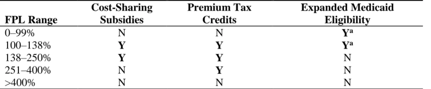
Table 3.1. ACA program eligibility ... 44
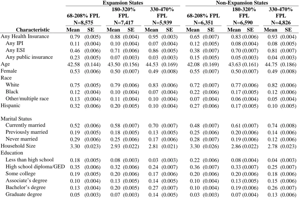
Table 3.2. Weighted summary statistics ... 45
Table 3.3. Regression discontinuity estimates at 138% FPL/100% FPL, 250% FPL, and 400% FPL for HI outcomes, 2014 ... 47
Table 3.4. RD estimates for expansion states at 138% FPL by key demographics, 2014 ... 48
Table 3.5. RD Estimates for non-expansion states at 100% FPL by key demographics, 2014 ... 49
Table 4.1. Summary statistics ... 93
Table 4.2. Summary statistics for FTFY sample by ESI status ... 96
Table 4.3. Summary statistics for PTPY sample by ESI status ... 99
Table 4.4. Summary statistics for the FULL sample by ESI status ... 102
Table 4.5. DD regression estimates by sample and referent group ... 105
Table 4.6. DDD regression estimates by sample and referent group ... 106
Appendix Table 1. Regression discontinuity estimates at 138% FPL/100% FPL, 250% FPL, and 400% FPL for HI outcomes, 2010–2012 ... 125
Appendix Table 2. Balance checks using inverse propensity score weighting ... 134
Appendix Table 3. Balance checks using entropy balance weighting ... 137
Appendix Table 4. Earnings dispersion between 1995 and 2012 ... 139
Appendix Table 5. FULL sample DD regression estimates with an interaction with FTFY status... 140
LIST OF FIGURES
Figure 2.1. RD estimates at the 300% FPL cutoff ... 12
Figure 3.1. FPL density estimates, post- and pre-2014... 50
Figure 3.2. Any HI coverage by 5% FPL bins in 2014... 51
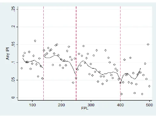
Figure 3.3. IPI coverage by 5% FPL bins in 2014 ... 52
Figure 3.4. ESI coverage by 5% FPL bins in 2014 ... 53
Figure 3.5. PHI coverage by 5% FPL bins in 2014 ... 54
Figure 3.6. Log non-zero HI premiums for IPI-covered individuals in 2014 ... 55
Figure 3.7. Log OOP expenditures for IPI-covered individuals in 2014 ... 56
Figure 4.1. Health insurance coverage, 1995–2012 ... 107
Figure 4.2. Log earnings by sample definition ... 108
Figure 4.3. Log earnings across ESI policy holders and referent groups, by sample definition ... 109
Figure 4.4. Log earnings change by percentile by sample, 1995 and 2007 ... 111
Figure 4.5. Log earnings change by percentile by sample and referent group, 1995 and 2007 ... 112
Figure 4.6. DD quantile regression estimates using binary ESI, 1995 and 2007, preferred FTFY models... 114
Figure 4.7. DD quantile regression estimates using binary ESI, 1995 and 2007, PTPY sample ... 115
Figure 4.8. DD quantile regression estimates using binary ESI, 1995 and 2007, FULL and quasi-experimental weighted samples ... 116
Figure 4.9. DD quantile regression estimates using employer and employee premiums, 1995 and 2007, preferred models ... 117
Figure 4.10. DD quantile regression estimates using employer and employee premiums, 1995 and 2007, non-preferred models ... 118
Appendix Figure 1. Density estimates around the 300% FPL cutoff, Massachusetts ... 121
Appendix Figure 3. Permutation tests for the post-period ... 123
Appendix Figure 4. Any HI coverage by 5% FPL bins in 2010–2012 ... 126
Appendix Figure 5. IPI coverage by 5% FPL bins in 2010–2012 ... 127
Appendix Figure 6. ESI coverage by 5% FPL bins in 2010–2012 ... 128
Appendix Figure 7. PHI coverage by 5% FPL bins in 2010-2012 ... 129
Appendix Figure 8. Permutation testing for different FPL cutoffs for the probability of having IPI in 2014, 38%-238% FPL ... 130
Appendix Figure 9. Permutation testing for different FPL cutoffs for the probability of having IPI in 2014, 150%-350% FPL ... 131
Appendix Figure 10. Permutation testing for different FPL cutoffs for the probability of having IPI in 2014, 300%-500% FPL ... 132
Appendix Figure 11. Bandwidth testing for the 138%/100% FPL cutoff for the probability of having IPI in 2014 ... 133
Appendix Figure 12. Log earnings at each percentile by sample, 1995 and 2007 ... 143
LIST OF ABBREVIATIONS
CPS: Current Population Survey ESI: employer-sponsored insurance FPL: federal poverty level
HI: health insurance
IPI: individually purchased insurance PHI: public health insurance
RD: regression discontinuity
ESI PH: Employer-sponsored insurance policy holder FTFY: Full-time, full year
PTPY: Part-time or part-year
FULL: refers to the sample of all workers, including both FTFY and PTPY workers FTFY-ESI: Refers to the sample of FTFY workers that are ESI PHs or ESI dependents PTPY-ESI: Refers to the sample of PTPY workers that are ESI PHs or ESI dependents CPS: Current Population Survey
CHAPTER 1: INTRODUCTION
Recent health reform policies in the United States (US) focus on increasing access to, improving the quality of, and reducing the cost of medical care. Access, quality and cost are in many ways governed by health insurance. Given rising medical costs, health insurance not only provides indemnity against unexpected health shocks but affordable access to basic and routine medical services. Health insurance in the US is predominately provided through employment, with more than 60% of the population covered by an employer-sponsored health insurance (ESI) plan (DeNavas et al. 2009). ESI is appealing in large part because it offers a significant price reduction relative to private, non-group market prices. Individuals without access to ESI must rely on a volatile and expensive non-group market, obtain coverage through a public program if eligible, or be uninsured. Thus, although the Patient Protection and Affordable Care Act of 2010 (ACA) requires that employers offer health insurance, a major push of the ACA is to increase the availability and affordability of insurance through public insurance coverage expansions and through subsidy programs for private non-group insurance available on online marketplaces.
subsidies represent the broadest offering of subsidies for non-group health insurance. The ACA subsidies build on the subsidy plan first offered in Massachusetts as part of an earlier health reform in 2006.
There is limited evidence of the effectiveness of insurance subsidies for private, non-group health insurance. Existing subsidies are largely built into the tax system, providing general deductions for health care costs above 7.5% of adjusted gross income or more specific
deductions (e.g., the self-employed). Two recent studies focused on subsidies available to the self-employed (tax-based) and those recently unemployed (not tax-based) and have found modest, positive effects on insurance coverage (Heim & Lurie 2009, Moriya & Simon 2016).
In the context of the ACA, while eligible individuals receive a substantial subsidy, the monthly premiums may still be higher than individuals are willing to pay. Additionally, the search costs of navigating the exchanges may provide additional disincentive. By examining the effectiveness of the tax credits and cost-sharing combined and separately, this dissertation provides evidence on how consumers respond to differing levels of subsidies and how the incentives could be altered to increase participation. Two chapters in this dissertation examine the Massachusetts and broader ACA subsidy schemes.
More broadly, while the hypothetical tradeoff between ESI and earnings is well studied, the empirical evidence for a tradeoff is mixed and the mechanism by which increasing ESI premiums reduces wages is not well understood (Currie & Madrian 1999). ESI premiums increased more than 150% in the two decades prior to the implementation of the ACA and premiums markedly increased shortly after the ACA was passed. Since ESI remains the prevalent source of insurance coverage, the indirect consequences for earnings is an important consideration for policy makers. An offer of ESI voids eligibility for the ACA subsidies, which provides low- and middle-income little alternative to the coverage their employer offers in the face of an earnings tradeoff. As the existing literature focuses largely on the average effects of ESI premium increases on earnings, the third paper in this dissertation examines the
CHAPTER 2: DO PREMIUM TAX CREDITS INCREASE PRIVATE HEALTH INSURANCE COVERAGE? EVIDENCE FROM THE 2006 MASSACHUSETTS
HEALTH CARE REFORM Introduction
The costs of health care and health insurance (HI) have increased dramatically over the past several decades in the United States. Many individuals and families have relied on
employer-sponsored insurance (ESI) for affordable HI, but ESI has eroded recently as costs climb. To attempt to address this, many states have expanded public health insurance (PHI) to cover low-income families. In 2006, Massachusetts implemented a novel health reform that provided a marketplace for individuals to purchase HI directly. The marketplace was coupled with an individual mandate that ensured a large enough risk pool to contain premiums. To further incentivize participation, Massachusetts subsidized premiums for individuals below 300% of the federal poverty level (FPL).
Extensive literature has examined the broad impact of the Massachusetts reforms on the insured rate (e.g., Pande et al., 2011) and a variety of health and health care utilization outcomes (e.g., Kolstad & Kowalski, 2012). A methodological difficulty with such an extensive set of policies is to isolate the effects of different policy components. No study to date has looked directly at the tax credits. This study uses regression discontinuity (RD) to compare non-group private insurance coverage of individuals just below 300% FPL who were eligible for a tax credit to individuals just above who were not eligible.
and their effect has little empirical evidence. Evidence to date has focused on individuals who are laid off or are self-employed, and associated subsidies have produced modest, positive impacts. Given static premium costs, some consumers may not want HI regardless of the subsidy, and some may want it without a subsidy. From a policy maker’s perspective, the population of interest is those on the margin of purchasing insurance. The tax credit must be large enough to encourage participation for consumers who want insurance but not at pre-reform prices. I test whether the tax credits were large enough to increase participation.
Materials and Methods
The Current Population Survey (CPS) was chosen because it captures income, HI, and demographics before and after the 2006 Massachusetts health reform (Flood et al., 2015). The pre-reform period comprises calendar years 1999 through 2006, and the post-reform period comprises calendar years 2007 through 2009. The sample includes adults aged 18 to 64 and excludes veterans and individuals with imputed HI responses.
Although individuals can report multiple types of HI in a year, I used three exclusive categories for HI based on guidance from the literature: the primary outcome, individually purchased insurance (IPI); ESI; and PHI. If an individual reports ESI, they are excluded from being in the IPI or PHI. Individuals who report any ESI or IPI are not included in the PHI.
self-I estimated the RD model at 300% FPL using both parametric and nonparametric models. The base parametric specification is:
𝐻𝐼𝑖 = 𝛼 + 𝛽1𝑆𝑈𝐵(𝐹𝑃𝐿 < 300) 𝑖 + 𝛽2𝐹𝑃𝐿(𝑥 − 300)𝑖+ 𝛽3𝑆𝑈𝐵(𝐹𝑃𝐿 < 300) 𝑖
∗ 𝐹𝑃𝐿(𝑥 − 300)𝑖 + 𝛿𝑿𝑖 + 𝜏𝑖+ 𝜀𝑖
where HI is a binary HI indicator, SUB is a binary indicator for below 300% FPL. FPL is centered at 300%, 𝑿is a vector of individual demographics described above, and 𝜏𝑖 are year fixed effects. 𝜀𝑖 is assumed to be an independently and identically distributed error term. 𝛽1 is the treatment effect at the discontinuity. All models use the HI-specific probability weight. I estimate the above equation with and without 𝑿 and 𝜏𝑖 and with higher-order FPL terms. Standard errors are clustered on the FPL for the parametric models (Lee & Card, 2008). I also pooled each model and computed a difference-in-differences effect at the cutoff. Lastly, a non-parametric RD was estimated using local linear regression with a triangle kernel density estimator.
Following Imbens and Lemieux (2008), four sensitivity and falsification tests were used to test the robustness of the results: checking for false cutoffs, changing the bandwidth around the cutoff, McCrary’s (2008) test manipulation of the forcing variable, and discontinuities in demographic characteristics. An additional test examined nonrandom heaping (Barecca et al., 2011). The sensitivity tests do not meaningfully alter the results of this study.
cutoff is determined by family size, this creates lumpiness in the histogram (see Online Appendix Figures 1 and 2).
Results
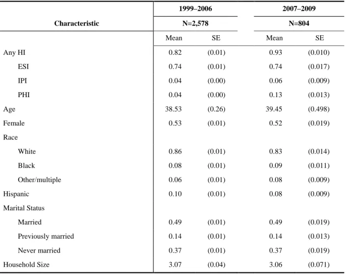
Table 2.1 presents weighted summary statistics for the 1999–2006 and 2007–2009 samples between 230% and 370% FPL. The summary statistics demonstrated a slight increase in IPI and PHI across time. There was little change in demographic characteristics of the sample across time, including education and self-reported health (not presented).
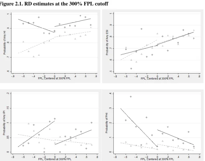
Figure 2.1 presents the main RD results graphically for the post-reform periods for all outcomes, and Table 2.2 presents statistical estimates for the effect shown in Figure 2.1. The bottom left panel of Figure 2.1 shows an increase in IPI just below 300% FPL in the post-reform period and no detectable effect in the pre-reform period. The nonparametric estimates for IPI are a statistically significant increase of 8.4 percentage points, and the cubic model estimates a 19.4 percentage point effect. The linear and difference-in-differences models are similar in magnitude to the non-parametric model, but they are not statistically significant.
Although IPI is the primary outcome, the remainder of Figure 2.1 and Table 2.2 present the broader effects on other HI outcomes. The upper left panel of Figure 2.1 shows that any HI coverage decreased slightly in the post-reform period just below 300% FPL. The estimate for that effect was 4 to 5 percentage points, and it was not statistically significant. Although
imprecise, this result suggests that the increase in coverage in IPI due to the subsidies was offset by a general decrease in coverage.
more noise. Still, Table 2.2 suggests that the reduction in PHI was statistically significant in the post-reform period, ranging in effect size from 12 to 18 percentage points.
One potential explanation for the overall decrease in HI and large decrease in PHI is crowd-out. However, there were not concurrent Medicaid policy changes at 300% FPL. These effects could instead be explained by volatility between ESI and PHI due to the Great Recession. For the bin proportions of ESI and PHI in Figure 2.1, spikes in ESI coverage line up with
decreases in PHI and vice versa. There were not enough observations to test this hypothesis by looking at years separately.
The permutation testing also provided a meaningful check for interpreting the ESI/PHI effect. The effect for IPI was largest in magnitude and the test statistic relative to all surrounding points in the FPL distribution (see Online Appendix Figure 3), suggesting a valid treatment effect. The permutation tests were much less clear for ESI and PHI where there were large effects in both directions at multiple false cutoffs between 220% and 300% FPL, suggesting the large PHI effects seen at 300% were not associated with the tax credits.
Discussion
This study examined the effectiveness of premium tax credits on IPI associated with the 2006 Massachusetts health reform. I find evidence of an increase in IPI participation among those below the 300% FPL cutoff at which individuals become ineligible for subsidized insurance but a statistically insignificant decrease in any HI coverage.
as PHI or vice versa, given the strong advocacy and state-branding that occurred with health reform.
Tables
Table 2.1 Weighted summary statistics, 230%–370% FPL
1999–2006 2007–2009
Characteristic N=2,578 N=804
Mean SE Mean SE
Any HI 0.82 (0.01) 0.93 (0.010)
ESI 0.74 (0.01) 0.74 (0.017)
IPI 0.04 (0.00) 0.06 (0.009)
PHI 0.04 (0.00) 0.13 (0.013)
Age 38.53 (0.26) 39.45 (0.498)
Female 0.53 (0.01) 0.52 (0.019)
Race
White 0.86 (0.01) 0.83 (0.014)
Black 0.08 (0.01) 0.09 (0.011)
Other/multiple 0.06 (0.01) 0.08 (0.009)
Hispanic 0.10 (0.01) 0.08 (0.009)
Marital Status
Married 0.49 (0.01) 0.49 (0.019)
Previously married 0.14 (0.01) 0.14 (0.013)
Never married 0.37 (0.01) 0.37 (0.019)
Household Size 3.07 (0.04) 3.06 (0.071)
Table 2.2. Regressions discontinuity estimates of health insurance uptake at 300% FPL
Post-Reform: 2007–2009 Pre-Reform: 1999–2006
Difference-in-Differences
Non-parametric Linear Cubic
Non-parametric Linear Cubic Linear Cubic Any HI −0.048 −0.041 −0.128 0.008 −0.021 0.010 −0.068 −0.049
(0.051) (0.055) (0.104) (0.032) (0.034) (0.063) (0.075) (0.143)
Any IPI 0.084** 0.070 0.194** −0.002 −0.003 0.050 0.082 0.161
(0.039) (0.043) (0.092) (0.017) (0.020) (0.033) (0.057) (0.120)
Any ESI −0.013 0.044 −0.132 0.043 0.014 0.032 −0.031 −0.054
(0.072) (0.082) (0.161) (0.036) (0.039) (0.075) (0.101) (0.205)
Any PHI −0.118** −0.155*** −0.186* −0.038** −0.032* −0.070 −0.119* −0.155
(0.049) (0.056) (0.098) (0.016) (0.019) (0.043) (0.063) (0.113)
Figures
Figure 2.1. RD estimates at the 300% FPL cutoff
CHAPTER 3: INCENTIVE(LESS)? THE EFFECTIVENESS OF TAX CREDITS AND COST-SHARING SUBSIDIES IN THE AFFORDABLE CARE ACT
Introduction
The Patient Protection and Affordable Care Act of 2010 (ACA) implemented a complex, broad set of changes in the U.S. health insurance and health care system. In 2014, several
prominent ACA components went into effect. First, insurance mandates require individuals to obtain and large employers to offer coverage or pay a penalty. Second, states could choose to expand Medicaid eligibility to childless, low-income adults. Third, individuals could purchase private insurance through online marketplaces and a receive a subsidy in the form of advance premium tax credits (APTCs) and cost-sharing reductions (CSRs) if the income falls between 100% and 400% of the Federal Poverty Level (FPL). APTCs reduce monthly premium payments and CSRs reduce certain elements of cost-sharing, such as co-payments or out-of-pocket
maximums. The amount of the APTCs and CSRs vary considerably between 100% and 400% FPL.
insured rate but the other components, including the APTCs and CSRs, contribute substantially to the increase in the insured rate as well.
Beyond the policy impact on the overall insured rate, the APTCs and CSRs provide an opportunity to better understand the elasticity of demand for health insurance. Tax credits have been used in the past to incentivize employer-sponsored insurance (ESI) coverage (e.g., Moriya and Simon 2016) and individually purchased insurance (IPI) among the self-employed (e.g., Heim and Lurie 2009), and have typically yielded relatively low elasticities between 0.6 and -0.3. Under the ACA, the APTCs and CSRs represent a large expansion of tax credits to a low-income population, for which there are few elasticity estimates.
In this study, I exploit the discrete changes in eligibility by income relative to the FPL with a regression discontinuity (RD) design to identify the combined and separate effects of the APTCs and CSRs. Individuals gain eligibility for both APTCs and CSRs at 100% FPL, lose eligibility for CSRs at 250% FPL, and lose eligibility for the APTCs at 400% FPL. In Medicaid expansion states, individuals initially gain eligibility at 138% FPL instead of 100% FPL in non-expansion states. This creates three plausibly exogenous cutoffs where subsidy eligibility changes dramatically: 138%/100% FPL with highly subsidized APTCs and CSRs; 250% FPL where CSRs are no longer available; and 400% FPL where APTCs are no longer available. In this way, the lowest cutoff tests the combined APTC/CSR subsidy, the middle cutoff tests for changes associated with the CSRs, and the highest cutoff tests for an APTC-only effect.
evidence of bunching around the cutoffs. Prior studies focusing on the Massachusetts reform use RD and find no evidence of income manipulation (Hinde 2016, Chandra, Gruber and McKnight 2010, 2014). In contrast to other studies that examine APTCs and CSRs, I use an income
definition more consistent with actual APTC/CSR eligibility. The design also does not require the identification of control group, which is problematic for ACA studies using difference-in-differences given the widespread reach of the ACA. By focusing on the discrete changes at each cutoff, it possible to separately examine the APTCs from the CSRs.
I find strong evidence of a 4.8 to 5.4 percentage point increase in IPI just above 138% FPL in Medicaid expansion states, where subsidized insurance coverage is first available and individuals are just ineligible for the expanded Medicaid program. At the 138% FPL cutoff, I estimate an elasticity of demand for health insurance ranging from -0.65 to -0.58. In non-expansion states, the effects above 100% FPL are slightly smaller in magnitude and not statistically significant for the general population, but is instead concentrated among 20-to-39 year olds. There is no evidence of an effect at the 250% FPL cutoff attributable solely to the CSRs. I do find suggestive evidence of an increase in IPI at the 400% FPL cutoff attributable to the APTC in states that implemented a state-based exchange.
health insurance (PHI) for married individuals and employer-sponsored insurance (ESI) for non-married individuals.
While similar tax credits have been used in past programs related to self-employment and for recently unemployed individuals, the results here suggest that these ACA tax credits may have broader appeal for lower-income individuals. The estimated elasticities are also on the high end of existing estimates, suggesting low-income individuals may be more price responsive than previous studies have found. There is no evidence for changes in IPI coverage at 250% FPL and weak evidence for changes at 400% FPL, consistent with existing low elasticity estimates for higher income individuals.
One policy implication is that the APTC and CSR levels would need to be raised at higher incomes to induce more participation. Furthermore, these results suggest the long-term impact beyond the lowest-income group could be minimal. However, given that the individual mandate penalty and the exchange premium increases in 2015 could further incentivize
participation, consumer awareness of and responsiveness to these changes are a key determinant of how much the APTC and CSR levels would need to be raised in the future.
Background
Institutional Setting
The primary focus of this analysis is to examine the impact of APTCs and CSRs that are available first in 2014 to certain income bands of the population and are obtained through state-based exchanges (SBE) or a federally-facilitated exchange (FFE). The ACA initiated HI
states opted for a partnership arrangement, whereby the state incorporated some components of the SBE but still deferred to the FFE for the enrollment process. In 2014, 17 states chose SBEs, 27 chose FFEs, and 7 chose a partnership arrangement.
To increase affordability of exchange plans, the ACA subsidized premiums to a varying degree for individuals with incomes between 100% and 400% of the FPL. The ACA
implemented APTCs for individuals between 100% and 400% FPL and CSRs for individuals between 100% and 250% FPL. For 2014, income thresholds for single individuals were $11,490 (100% FPL), $15,856 (138% FPL), $28,725 ($250% FPL) and $45,960 (400% FPL) (KFF, 2014a). The value of APTCs fall on a sliding scale, where individuals receive a higher relative subsidy at lower income levels. At 400% FPL, the income cap in 2014 was 9.5%, yielding a $4,320 maximum annual premium for an individual, or $363 monthly. At the bottom end at 100% FPL, the cap was 2%, yielding a maximum annual premium of $230, or $20 monthly. The amount of the APTC was the difference between the total annual premium and the income cap and was normalized to the price of the second lowest silver tier plan, so that individuals did not receive a higher subsidy for choosing a gold or platinum tier plan. The APTC could be applied at the time of enrollment to reduce monthly payments (referred to as the advanced premium tax credit) or collected in a lump sum through income tax filings. In 2014, 85% of consumers who enrolled in the exchange received the APTC (ASPE 2014).
The CSR subsidy was available to individuals between 100% and 250% FPL and
associated with the plan. For example, an exchange plan might have had a $2,000 deductible, a $6,400 out-of-pocket maximum, and a $45 co-payment for primary care physician visits. For an individual with income between 150%–200% FPL, the cost-sharing subsidy would have reduced the deductible to $500, the out-of-pocket maximum was capped at $2,250, and the co-payment is reduced to $15. Other than regulations on the out-of-pocket maximum, insurers could choose how to balance the deductible/co-payment mix to achieve an actuarial value of 87% for the 150%–200% FPL cost-sharing subsidy.
In this analysis, I focus on consumer health insurance decisions around each of three eligibility cutoffs: 100%/138% FPL, 250% FPL, and 400% FPL. Table 3.1 describes how program eligibility changes across the different FPL cutoffs. I use 138% FPL for Medicaid expansion states instead of 100% FPL to avoid overlap with expanded Medicaid eligibility. The RD design compares individuals just above and below each of the three FPL cutoffs. In what follows, I refer to changes around the 100%/138% FPL cutoffs as a combined effect of the APTCs and CSRs. Just above 100%/138% FPL, individuals gain eligibility to the dual incentive. For expansion states, those who fall below 138% FPL are potentially eligible for Medicaid, so this effect may be capturing changes in preferences between public and private coverage. In non-expansion states, a coverage gap exists, where individuals below 100% FPL have no access to APTCs/CSRs and are unlikely to be newly eligible for Medicaid. Thus, the incentive is different and potentially much more valuable in non-expansion states.
the 400% FPL cutoff as the effect of the APTC only, comparing individuals just below 400% FPL that are eligible for APTCs and individuals just above 400% FPL that are ineligible.
A second incentive to health insurance participation is an individual mandate that
requires all individuals to obtain a minimum 60% actuarial value HI plan or pay a lump sum tax ($95 or 1% of income per adult in 2014, $325 per adult in 2015, and $695 per adult in 2016) (KFF, 2014b). Furthermore, the penalty is not applied to individuals with incomes that fall below the tax filing threshold or 138% FPL in states that do not expand Medicaid, Native Americans, or if the lowest exchange premium available is greater than 8% of income. Given the low level of the tax in 2014, the contamination of this component is assumed to be zero for this analysis. This is consistent with preliminary evidence that the mandate had little effect on insurance coverage (Frean, Gruber, and Sommers, 2016).
This analysis does not formally examine Medicaid expansion, which extends Medicaid eligibility to childless adults under 138% FPL. Medicaid expansion interacts with the analyses here, since many individuals are newly eligible just below 138% FPL. An intended effect of the research design is that many individuals should lose eligibility for Medicaid coverage above 138% FPL in states that choose to expand. This is not a policy effect in the context of the current study in as much as a validity check.
Prior Literature
with an income 138%–399% FPL through June 2014 and a 7.4 percentage point increase through March 2015 (Long et al., 2014, 2015). The gains vary by age, race/ethnicity, and gender and are potentially larger in Medicaid expansion states. Among those uninsured between 138%–399% FPL, almost half of respondents were unaware of the incentives, approximately 60% were uninsured primarily due to costs of insurance, and 20% did not want insurance or would rather pay the nonparticipation fine (Shartzer et al., 2014). Estimates from the Gallup Poll and National Health Interview Survey find similar reductions in the proportion of uninsured (e.g., Black and Cohen, 2014; Sommers et al., 2015).
Two recent studies use a triple difference method, taking advantage of pre-2014 variation in the local area uninsured rate, to separate the effects of the different ACA components on insurance coverage. Courtemanche et al. (2016) use cross-state variation in Medicaid expansion status and estimate a 5.9 percentage point increase in the insured rate. They attribute half of the increase to Medicaid expansion and the other half to ACA components. Frean, Gruber and Sommers (2016) use variation in premiums across geographic regions to separate the effects of APTCs, individual mandate, and Medicaid expansion. They find the APTCs account for 37% of the observed reduction in the uninsured rate and Medicaid expansion accounts for 63%. They further describe that most of the Medicaid expansion effects are driven by a woodwork effect – increased uptake by previously eligible individuals. For the APTCs, Frean, Gruber and Sommers (2016) estimate a small average price elasticity of -0.05. While Courtemanche et al. (2016) find evidence for a partial crowding out of public insurance, Frean, Gruber and Sommers (2016) find no evidence of crowding out.
Other quasi-experimental analyses of specific ACA components focus on early
mandate. For example, Golberstein et al. (2015) find large increases in public HI (PHI) coverage associated with Medicaid expansion in California. Kaestner and colleagues (2015) used
difference-in-differences and synthetic control methods to estimate an approximately 4 percentage point increase in PHI due to early Medicaid expansions. Evidence from the dependent-coverage mandate indicates a marked increase in insurance coverage among those less than 26 years of age (e.g., Antwi et al., 2013).
Several other studies examine the impact of the ACA on ESI. Survey data from the Urban Institute show little evidence of changes in ESI availability, ESI take-up, and ESI coverage, but offer suggestive evidence that ESI coverage increases for employees of small employers and low incomes (Blavin et al., 2015). The 2015 Employer Health Benefits Survey indicates an increase in ESI premiums consistent with increases from previous years and notes little change in benefit design (Claxton et al. 2015). The rapid response surveys provide suggestive evidence of
anticipatory changes in offer and benefit design to meet ACA requirements, but little overall impact on ESI.
relevant base for the elasticity estimate should be the total premium cost. This shift in thought suggests the early estimates are potentially low (e.g., Baicker and Chandra 2006).
For non-ESI elasticities, another literature focuses on subsidies for self-employed and recently unemployed. Gruber and Poterba (1994) compare how changes in tax deductibility affect insurance among self-employed individuals compared to employed individuals and estimate an elasticity between -3 and -1. Using an individual fixed effects model, a more recent study by Heim and Lurie (2009) estimates a smaller elasticity for the selfemployed, between -0.6 and -0.3. The American Recovery and Reinvestment Act of 2008 provided health insurance subsidies to recently unemployed individuals who previously had access to ESI. The ARRA subsidy lets individuals pay 35 percent of the full ESI premium while the employer is repaid 65 percent of the subsidy by the government. Moriya and Simon (2016) estimate an elasticity of -0.38 to -0.27. These studies yield moderate price elasticities for narrowly defined populations – self-employed and recently unemployed individuals. The APTC apply to a broader portion of the population, and a potentially different population – lower-income individuals.
services, similar to the elasticity estimated in the seminal RAND Health Insurance Experiment (Newhouse 1993).
A recent working paper by Pauly et al. (2015) simulates financial implications and welfare changes associated with the 2014 APTCs and CSRs. Their results indicate that the additional financial burden of purchasing HI are offset by increases in welfare due to expected medical care prices for individuals below 250%. Aligning with these projections, I hypothesize the effects may be strongest at 100%/138% and 250%, where consumers have access to the APTCs and CSRs. Combined with the low elasticity estimate from Chandra, Gruber and
McKnight (2014), the effect at 250% FPL is likely to be weaker, since the change in the CSR is lower across that cutoff.
Methods
Data
are developed to correct for differences in the series (Pascale et al. 2016). Therefore, the pre-period cannot currently be used as a baseline for 2014 changes. Furthermore, I exclude calendar year 2013 from the pre-period due to concerns about respondents reporting current coverage as of March 2014 instead of past year coverage (Swartz 1986).
The analytic sample includes adults aged 26 to 64. Individuals over 64 are almost
universally covered by Medicare. Any individual with an allocated HI status is also dropped; HI status is allocated for some respondents based on other answers and information on the
respondent’s record or imputed if the interview was not fully completed. Allocation does not include logical imputation for PHI. Lastly, I also drop respondents residing in Massachusetts due to pre-existing health reform policies that directly overlap with the ACA policies.
The main outcome is past year HI status. I measure whether respondents had any HI and four exclusive categories of HI: IPI, ESI, and PHI, or uninsured. If an individual reports ESI coverage during a given year, he or she is not assigned IPI or PHI. Individuals who report any ESI or IPI are not assigned PHI. The primary independent variable is the respondent’s income relative to the FPL. FPL is the ratio of the total family income to the federally determined
poverty threshold. The poverty threshold is based on the size of the family. Binary indicators are used to denote incomes that fell below 400% and 250% and above 100%/138% FPL; these capture the eligibility cutoffs for different components of the ACA in the RD design. As noted, there is a difference in the lowest cutoff between expansion (138% FPL) and non-expansion states (100% FPL).
matching with Internal Revenue Service (IRS) tax records (O’Hara 2004). AGI removes certain tax deductions and exemptions from gross income; AGI is lower than gross income. MAGI includes foreign-earned income, tax-exempt interest and non-taxable social security benefits. At lower income levels, the difference between MAGI and AGI is likely small.1 Statistical matching
introduces a potential source of measurement error, but there are not better sources that capture AGI beyond the IRS data (conversely, the IRS data do not historically measure broader HI coverage well). To account for differences between MAGI and AGI, all models exclude observations within 1% FPL of the cutoff to conservatively estimate the policy effects. The results are not sensitive to alternative models that include observations within 1% FPL
The AGI statistical match is made on household heads. I logically assign the imputed AGI to household members since the eligibility decision is made at the household level. The results do not change if only household heads are used. Rather, the standard errors improve, providing indirect evidence of measurement error. The results presented here are conservative.
A series of covariates are also used to control for potential confounding factors: age, gender, race, ethnicity, marital status, family size, living in a metropolitan statistical area,
education, self-reported health status, Census region, and state of residence. Age and family size are treated as continuous variables, while binary indicators are used for the remaining individual controls.
1 Based on author’s calculations using the 2014 IRS SOI
Empirical Methods
To estimate the effects of the APTCs and CSRs on coverage, a sharp RD design is applied using the 100%/138%, 250%, and 400% FPL cutoffs in 2014 as exogenous forcing variables.2 The estimation approach logically separates the sample into two groups: expansion
and non-expansion states. The 138% cutoff only applies to expansion states, and the 100% FPL cutoff to non-expansion states, requiring separation when examining the lowest cutoff. Twenty-eight states expanded Medicaid by 2014 to include childless adults below 138% FPL.
RD compares individuals just below and just above each FPL cutoff, assuming that the only difference between individuals is eligibility for the APTCs, CSRs, or Medicaid. Hinde (2016) uses exact design and data source to estimate the impact of the tax credits available below 300% FPL in Massachusetts in 2006 (Hinde 2016) and Chandra, Gruber and McKnight (2010, 2014) use FPL cutoffs as an exogenous source of variation to examine CSRs used in the 2006 Massachusetts reform.
RD is first estimated non-parametrically using local linear regression with a triangle kernel density estimator. Multiple bandwidths are used for the local linear estimation to examine sensitivity to the bandwidth (Lee and Lemieux 2010). RD is also estimated using a standard linear specification. The following specification references the 100% FPL cutoff, but applies similarly to the other cutoffs.3
2 One could argue that a fuzzy RD would be better in this context given the measurement errors concerns described
in the previous section. For a fuzzy RD design, one would need to know whether an individual receives APTC and CSR subsidies to serve as the first-stage outcome. Since the CPS does not capture whether or not an individual receives the APTCs and CSRs, the outcome for the first-stage is missing and a fuzzy RD is not possible.
3 For the 250% and 400% FPL cutoff, the SUB variable refers to being just below the cutoff, reversing the inequality
𝐻𝐼𝑖 = 𝛼 + 𝛽1𝑆𝑈𝐵(𝐹𝑃𝐿 > 100) 𝑖 + 𝛽2𝐹𝑃𝐿(𝑥 − 100)𝑖+ 𝛽3𝑆𝑈𝐵(𝐹𝑃𝐿 > 100) 𝑖
∗ 𝐹𝑃𝐿(𝑥 − 100)𝑖 + 𝛿𝑿𝑖 + 𝛾𝑠+ 𝜀𝑖
where HI is a binary HI indicator, and SUB is a binary indicator for above 100% FPL, FPL is centered at 100% FPL, 𝑿is a vector of the individual demographics described above, and 𝛾𝑠 are state fixed effects. 𝜀𝑖 is assumed to be an independently and identically distributed error term. The FPL cutoff indicator and the continuous FPL measure are interacted to allow the slope of the FPL trend to vary on either side of the cutoff. 𝛽1 represents the treatment effect at the
discontinuity. The nonparametric model estimates the equivalent of 𝛽1 but without imposing linearity of trends. I report detailed treatment effects for any HI and IPI, the categories directly affected by the APTCs and CSRs. For completeness, I also report estimates for ESI and PHI. The above equation is also estimated for the pre-period separately and presented in Appendix Table 1 and Appendix Figures 4 to 7. Pre-period estimates include year fixed effects.
To test for improvements in fit of the parametric form, I use higher order FPL terms in the parametric model. Models are estimated with and without the vector of individual-level controls. The models are not generally sensitive to higher order terms or covariate inclusion. Standard errors are clustered on the FPL for all models, as recommended by Lee and Card (2008) to account for the potential discreteness of the forcing variable. Results are not sensitive to alternative standard error calculations, such as heteroscedastic-robust standard errors or
A potential concern with this application of RD is that income can be manipulated, which would threaten identification. Historically, programs enforced through the tax code, such as the EITC, have been known to cause kink points in the income distribution (e.g., Saez 2010). Unlike other tax-based policies, such as the EITC, the APTC and CSR are not pure income transfers. In this context, there is also a temporal disconnect between the enrollment decision and tax
reconciliation. The enrollment period for the exchanges occurs in the fall months prior to the beginning of the next calendar year.4 Thus, individuals prospectively decide to enroll based on
projected income. The final amount of the APTC is not determined until tax filing the following year, where a repayment penalty occurs if individuals underestimate income.
The RD design is focused on the availability of the APTCs and CSRs at certain FPL thresholds, not the actual receipt of the incentives. To manipulate income to maintain eligibility, one could alter labor supply to affect earnings or take advantage of various tax credits and deductions, such as individual retirement account contributions, at tax filing to get under a threshold. To test for this type of manipulation, I look for evidence of income bunching around the FPL thresholds and changes in labor market behavior. I also estimate the McCrary (2008) test for discontinuities in the distribution near the cutoffs. To preview results of the manipulation tests, I do not find evidence that incomes are manipulated and argue that the design is valid given the prospective nature of the enrollment decision. This is consistent with a previous study on the Massachusetts reform (Hinde 2016).
Four other standard sensitivity and falsification tests are used to test the robustness of the results (Imbens and Lemieux, 2008). First, I use a search procedure to move the cutoff around arbitrarily and test for treatment effects. The “false” cutoffs should have smaller treatment effects
in absolute magnitude and smaller test statistics than the actual cutoff (Imbens and Lemieux, 2008). The cutoff is arbitrarily moved from 38% FPL to 238% FPL, 150% FPL to 250% FPL, and 300% FPL to 500% FPL in 5% increments, and potential discontinuities were examined at each arbitrary cutoff.
Second, different bandwidths around the cutoffs are tested to examine the sensitivity of the results to bandwidth selection. There is no theoretical guidance on optimal bandwidth selection. There is a tradeoff between bias and precision in determining the bandwidth: wider bandwidths are more likely to be biased and are more precise, whereas narrower bandwidths are less likely to be biased and are less precise. The selected bandwidth is 70%, and the bandwidth is allowed to vary between 25% and 100%.
Third, I examine nonrandom heaping with the FPL, a concern raised by Barreca et al. (2011, 2012; see also Almond et al., 2011). This test deals with the fact that respondents tend to report income in $1,000 or $10,000 increments, potentially leading to blips in the disaggregated data series. This is distinct from a discontinuity in the density of the sample distribution, which may indicate manipulation of the forcing variable. Nonrandom heaping close to the cutoff can potentially bias the treatment effects. Barreca et al. (2011) recommend a donut-hole RD, where the heap is dropped from the estimation procedure. The exclusion of observations within 1% FPL constitutes a donut-hole RD.
Results
Main Results
Table 3.2 presents summary statistics around each cutoff for expansion and non-expansion states, respectively. Across all states, any HI and ESI coverage increases as income increases, while IPI decreases slightly from the lower to higher incomes. Across both expansion and non-expansion states, IPI coverage is similar at each cutoff. The main difference in HI coverage across expansion and non-expansion states comes from the 8 percentage point difference for PHI around 138% FPL in expansion states. There are some minor differences in other demographic characteristics between lower and high incomes. Namely, as income increases individuals are more likely be older, married, white, and well-educated.
A critical assumption for an RD design is that there is no manipulation in the forcing variable. This assumption can be visually assessed with histograms by checking for
discontinuities in the FPL sample distribution at the cutoff and estimating the McCrary (2008) test for manipulation. Figure 3.1 presents a histogram for the expansion and non-expansion states for 2010-2012 and 2014. There is no visual evidence of mass points occurring near the cutoffs that would indicate manipulation nor large changes across time. Likewise, the McCrary test does not indicate large or significant differences in the FPL density at any cutoff. To further assess manipulation, I examine labor market outcomes at each of the cutoffs, since altering labor supply is one way to alter income. I find no differences at the cutoffs in labor force participation,
unemployment, self-employment, or part-time status (results available upon request). There is no evidence of any income manipulation that would invalidate the RD design.
To visually assess the effects of the combined APTCs and CSRs, Figures 3.2 through 3.5 show HI coverage across the FPL distribution for the four types of HI. The hollow circle
figures also impose a local linear trend between the cutoffs to visualize potential treatment effects near the cutoffs.
In Figure 3.2, while the proportion with any HI increases over the FPL distribution, there are no clear breaks at any of the cutoffs, except for a potential dip in any HI coverage just below 250% FPL in non-expansion states. For expansion states in the top panel of Figure 3.3, there is a noticeable increase in the scatterplot just above 138% FPL and the local linear trends suggest a large, positive effect on IPI coverage relative to those below 138% FPL. Moving further above 138% FPL, the scatterplot and local linear curve trend downward until 400% FPL where it appeared to flatten out. There is no visual evidence of a treatment effect near 250% in the scatterplot, but the local linear curves indicate a small, negative effect just below 250% FPL. Near 400% FPL, the change in the FPL trends indicate a small, positive effect.
For non-expansion states in the bottom panel of Figure 3.3, the plot looks quite similar to expansion states. There is an apparent effect just above 100% FPL, similar in magnitude to the effect above 138% FPL in expansion states, although not as clean. Between 100% FPL and 250% FPL, the IPI trend declines until it flattens out above 250% FPL. There is a small, negative effect just below 250% FPL and just below 400% FPL according to the local linear trends, but again, the visual evidence for an effect is weak.
Statistical estimates of the treatment effects are presented in Table 3.3. For expansion states, there are negligible changes in any HI coverage at all three cutoffs. The overall changes in the insured rate are not statistically significant, and for expansion states, suggest a minimal level of crowding out from Medicaid expansion. The increase in IPI is offset by a 1.3 to 2.3 percentage point drop in ESI and a 3.1-3.2 percentage point drop in PHI. For IPI, the combined treatment effect just above 138% FPL in expansion states is 5.4 percentage points in the non-parametric model and 4.8 percentage points in the linear model. Both estimates are statistically significant. The proportion covered by IPI between 68% and 138% FPL in 2014 is 0.104. The percentage increase associated with the combined incentive, therefore, ranges from 46.6% to 52.5%. Per ASPE reports from the FFE, the APTC reduced the average premium by 80%, implying an elasticity ranging from -0.65 to -0.58 (ASPE 2014).
Among the non-expansion states, there is a non-parametric 4.3 percentage point effect and a linear 3.4 percentage point effect for any HI at 100% FPL, although it is insignificant. The combined incentive effect for IPI just above 100% FPL is a smaller 2.3 percentage points and statistically insignificant. However, there is a similar increase in ESI of 1.7 to 2.6 percentage points.
Confirming the visual evidence in Figure 3.3, I do not find evidence of an effect on any HI coverage or a cost-sharing treatment effect for IPI just below 250% FPL. For expansion states, there is an insignificant 1.3 percentage point reduction in IPI just below 250% FPL. There is a marginally significant drop in any HI coverage of 3.9 percentage points in
Contrary to the visual evidence of a positive effect just below 400% FPL in expansion states, the statistical estimate is positive but small and insignificant. A separate model focusing solely on the SBE states estimates a 3.6 percentage point increase in IPI just below 400% FPL and the effect was significant at the 10% level. Again, there is no evidence of any effects near 400% FPL in non-expansion states
In summary of the IPI results, I find strong evidence of a combined effect of the APTCs and CSRs just above 138% FPL in expansion states and less robust evidence of a combined effect just above 100% FPL in non-expansion states, where the incentives are strongest. There is no robust statistical evidence to support a CSR effect and only suggestive evidence of an APTC effect in SBE states. The positive effects for the combined incentive and APTC-only imply that the APTCs could be the driving incentive for consumers on the margin.
As a validity check, a separate set of analyses reproduce the main results for the 2010– 2012 period, available in Appendix Table 1 and Appendix Figures 4–6. No effects are found in the pre-period at 100%/138% FPL and 400% FPL. There is weak statistical evidence of a 2.4 percentage point increase in any HI coverage just below 250% FPL in expansion states and 1.5-1.6 percentage point increase in IPI just below 250% in non-expansion states. In both cases, there is not strong visual evidence of a jump in coverage. When disaggregated by year, all 3 effects dissipate. Given the sensitivity of the effects across years and the lack of visual evidence, there is little concern that the design is invalid for the 250% FPL cutoff.
Heterogeneous Effects
states are concentrated among a particular demographic, I stratify the models in Table 3.3 by three key characteristics: relationship status, self-reported health status, and age group. The estimates are presented in Table 3.4 for expansion states and Table 5 for non-expansion states.
Starting with expansion states in Table 3.4, there is a net increase in the insured rate for married individuals and a net decrease in non-married individuals. The combined effect of the APTCs and CSRs for IPI is slightly higher for married (approximately 5.5 percentage points) than non-married individuals (4.6 to 5.3 percentage points), but not practically different. The differences in any HI coverage across marital status is driven by ESI and PHI. There is a reduction of 5.9 to 6.2 percentage points in PHI for married individuals, whereas non-married individuals have a reduction in ESI of approximately 5.4 to 6.6 percentage points. The PHI drop-off is consistent with Medicaid ineligibility, but the ESI drop-drop-off for single individuals is
unexpected. This could be evidence of switching away from ESI toward IPI.
The next stratification is by self-reported health status, comparing individuals who reported being in excellent or very good health against individuals who reported being in good, fair, or poor health. Referring back to Table 3.2, there are too few individuals in fair and poor health to analyze separately. When stratified by health status, the combined effect is unchanged for the higher self-reported health group, and is somewhat attenuated for the lower self-reported health group for the linear specification. A reduction in PHI is observed only for the lower self-reported health group. Overall, there are negligible effects on the insured rate among the higher self-reported health or the lower self-reported health group. At least the extensive margin, there is no evidence of adverse selection in IPI take-up.
for the younger group and a negative, insignificant decrease in any HI in the older group. There is a small difference in the 3.6 to 4.7 percentage point combined effect and 5.8 to 6.1 percentage effect on IPI between younger and older groups, respectively. As with the marriage stratification, the older group experiences a reduction in PHI between 6.1 and 7 percentage points attributable to Medicaid ineligibility above 138% FPL, while the younger group does not see a
countervailing reduction in ESI comparable to the non-married group.
Table 3.4 provides three implications. First, there are only minor differences in the effect of the combined incentives on IPI across marital status and age group. Second, there is an
interesting dynamic of non-married individuals dropping off ESI coverage just above 138% FPL. Third, the non-married, older age groups see small net declines in the insured rate that are
associated with Medicaid ineligibility. In one sense, the results suggest that the desired effect of incentivizing, young, single and healthy individuals worked. In another sense, the net decrease in the insured rate for potentially vulnerable groups, signals a small crowding out effect.
For the non-expansion states in Table 3.5, there are three interesting findings. First, there is an increase in any HI for all groups except those reporting good, fair or poor health. Thus, the any HI significant for those in self-reported excellent or very good health is large, positive and significant. The 6.5 to 9 percentage point effect is driven by approximately equal increases in IPI and ESI. However, the increase in IPI and ESI is not significant. There is not the dynamic
tradeoff in ESI and PHI as with the expansion states and little evidence of crowd-out.
higher premium levels, the relative value of the subsidy should be higher for older adults and the lack of an effect is counterintuitive. It may point to issues in navigating the FFE and minimal outreach and navigational assistance in most non-expanding states, given the positive correlation between Medicaid expansion and adoption of a state-based exchange.
HI Premiums and Medical Spending
The results so far focus on the extensive margin of obtaining IPI. Beginning with the 2011 ASEC, respondents are asked to self-report HI premiums and out-of-pocket medical expenditures. The limited sample size in the CPS prevented in-depth statistical examination of the impact on premiums and out-of-pocket (OOP) medical expenditures conditional on having IPI. Instead, descriptive results of the impacts on premiums and OOP medical expenditures are presented. Figures 3.6 and 3.7 graphically present the average non-zero log premiums and log OOP spending for IPI-covered individuals before and after the exchanges and incentives went into effect in 2014, along with the local linear curves checking for discontinuities. These cost measures have not changed and are comparable across time, but are generally noisy.
Figure 3.6 shows that IPI premium payers in 2014 had lower average log premiums than 2010–2012 payers across the FPL distribution in both expansion and non-expansion states. For expansion states in 2014, the line is relatively smooth up to 250% FPL. Premiums drop slightly after 250% FPL and then exhibit a larger drop-off above 400% FPL. The trend lines are smooth in non-expansion states in 2014. For both state groupings, the pre-periods do not show large changes near any of the cutoffs.
converge back to pre-204 levels. This is suggestive of broader welfare benefits to consumers. There is also an increase in log OOP expenditures just below 400% FPL in expansion and non-expansion states in 2014. This last fact could be evidence of adverse selection. The demographic stratifications in Tables 3.4 and 3.5 do not suggest adverse selection on the extensive margin, but the effects below 400% FPL are weakly suggestive of adverse selection on the intensive margin. Robustness Checks
I implement a wide range of robustness checks and sensitivity analyses to attempt to refute the main results presented in the previous section. Results from the all robustness checks are summarized here. A selection of figures and tables for robustness checks are included in the Appendix and full results available upon request. The first robustness test involves arbitrarily moving the cutoff around the FPL distribution to create false cutoffs. The cutoffs near 138% or 100% FPL, 250%, and 400% FPL should have the largest effect size in absolute magnitude and the largest test statistic. There are no other large effects in the FPL range around 138% FPL for IPI in expansion states. Just above 100% FPL in non-expansion states there is a large, positive effect (see Appendix Figure 8). Near 250% FPL and 400% FPL for IPI in both expansion and non-expansion states, the permutation test is not suggestive of false effects (see Appendix Figures 95 and 10). Among the ESI and PHI outcomes, the permutation testing do not alter
interpretation of the main results at any cutoff.
The second robustness test alters the bandwidth for the model, ranging from 25% FPL on either side of the cutoff to 100% FPL on either side of the three cutoffs. There is no robust guidance on the appropriate bandwidth to use with an RD design. Should the results be sensitive
5Appendix Figure 8 also shows that there are no effects associated with the CSRs at 200% FPL in expansion states
to the bandwidth, it may cast doubt on the design. The results are appropriately sensitive to bandwidth selection (see Appendix Figure 11). Coefficient magnitude is at least constant or decreasing in absolute magnitude as the bandwidth increase.
The third robustness test assesses non-random heaping. I assess bunching using disaggregated scatter plots across FPL ranges for each outcome and do not find evidence of heaping.
The fourth and final robustness test examines potential effects of demographic shifts near the cutoffs. There is little visual evidence of demographic breaks near the cutoffs, but three demographic characteristics do have statistically significant differences in a few models: race/ethnicity, marital status, and family size. The proportion of non-white and Hispanic, not currently married, and average family size are noisy and decreasing in FPL in both expansion and non-expansion states, which help to explain why some models pick up a statistically significant effect. More importantly, the effects are small and there is no visual evidence of a demographic shift near any of the cutoffs.
Given the prospective incentives against cheating through repayment policies, the possibility of non-random measurement error is likely weakest in this study.6
A second limitation is that the data do not directly measure receipt of tax credits and cost-sharing subsidies or capture whether IPI is obtained through the exchanges. I assume that the cutoffs are binding and the demand for non-exchange coverage does not correlate with the ACA cutoffs. It is possible that non-exchange IPI coverage is wrapped up in the estimates. Built into this limitation is also the fact that the CPS income and HI questions were redesigned recently to better capture income and HI dynamics. Respondents could potentially confuse IPI coverage obtained through SBE exchanges or the FFE as PHI. As an anecdotal example, Kentucky and Colorado branded their exchanges as to not be associated with “Obamacare.” There may be some concern that the family size used in the FPL definition here exactly capture family size used in determining tax credit/cost-sharing eligibility. However, when the results are stratified by marital status in Table 3.5, the estimates are statistically indistinguishable.
As a final limitation, while the CPS provides a large sample size overall, using only 2014 data limits the relative sample size within FPL bins. The estimates could potentially be improved by additional years of data. The visual and statistical evidence support the main results of a combined effect, but more data is always better. In testing for income manipulation, I examine changes in labor market outcomes around the cutoffs. The null finding is consistent with other recent studies on the impacts of the ACA on labor markets (e.g., Gooptu et al., 2016). Given the precedence of income-based transfers affecting labor supply on the extensive and intensive
6 As noted earlier, individual retirement account contributions and other tax deductions/credits could be applied at
self-margins (e.g., Bitler et al. 2006), short-term labor responses may not be detectable with 2014 data alone, but should be monitored as more data become available. Future studies should examine whether long-term effects on labor market outcomes accrue.
Discussion
This analysis examines the effectiveness of ACA APTCs and CSRs implemented in 2014. Overall, the APTCs and CSRs are not associated with sharp changes in any HI coverage at any cutoff in expansion states, but are associated with insignificant, positive changes in any HI in non-expansion states. For IPI, however, I find robust, positive effects of the combined
APTC/CSR incentive just above 138% FPL in expansion states and weaker effects above 100% FPL in non-expansion states. This is a combined effect because consumers were initially eligible for APTCs and CSRs just above 138%/100% FPL. The APTC amount is highest and the CSR is most valuable at lower income levels, resulting in large effects where the incentives were strongest. Of particular policy importance is the finding that the increase in IPI in expansion states just above 138% FPL is offset by reductions in ESI and PHI. This suggests a minimal level of crowd-out and could have significant implications for public health care expenditures.
Despite the limitations noted in the previous section, the broad story painted by these estimates is a positive narrative of the initial effects of the combined incentive for lower income individuals. The difference in effect size and significance between expansion and non-expansion states also highlights previously identified coverage gaps among states opposing federal ACA policies. With a positive relationship between SBE adoption and Medicaid expansion, the
et al., 2015). Furthermore, many expanding states directly referred individuals to the SBE when ineligible for Medicaid. Consumers in non-SBE states still had access to the FFE, but they may not have had the same access to information and assistance as the SBE states (Dash et al., 2013; Long et al., 2015).
Tying into the broader literature examining the demand for health insurance, I estimate an elasticity of demand for health insurance of -0.65 to -0.58 for expansion states just above 138% FPL. This estimate is much larger than the -0.05 elasticity in Frean, Gruber and Sommers (2016), which is calculated using the average subsidy level (as in this study), but the treatment effect is for the broader 100-400% FPL population. Because the elasticity here is estimated on the margin of APTC and CSR eligibility, it suggests that low-income consumers on the margin are much more price-responsive than low-income individuals subject to the more gradual decline in the subsidy value.