Essays on retail operations

(1)

Essays on Retail Operations

by Olga Perdikaki

A dissertation submitted to the faculty of the University of North Carolina at Chapel Hill in partial fulﬁllment of the requirements for the degree of Doctor of Philosophy in the Kenan-Flagler Business School (Operations, Technology and Innovation Manage-ment).

Chapel Hill 2009

Approved by:

(2)

c

2009

(3)

ABSTRACT

OLGA PERDIKAKI: Essays on Retail Operations. (Under the direction of Dr. Jayashankar M. Swaminathan.)

The intensiﬁed competition that the retail industry faces with the increasing

num-bers of new players in both the local and global markets has forced retailers to critically

examine and redesign their operations and marketing strategies. To remain

competi-tive, many retailers have focused on the provision of enhanced customer experience and

pursued practices of diﬀerentiation. In this dissertation comprising of three essays, we

attempt to shed light on retail practices that enhance consumer valuation, on factors

that aﬀect store performance, and on temporal management of demand enhancing

ac-tivities using both analytical and empirical methodologies. The aim of this research is

to develop theoretical insights to help retailers understand their store performance and

eﬀectively manage strategies geared towards enhancing demand and consumer

valua-tion about their product oﬀerings.

In the ﬁrst essay, we focus on technology investments that can aﬀect consumer

valuation. We examine the impact of such investments in a duopoly setting in which

retailers compete in prices and consumers can search among the two retailers. In the

second essay, we focus on store performance and examine the impact of labor and

traﬃc characteristics on diﬀerent store performance metrics using proprietary data of a

retail chain. In the third essay, we focus on general services that retailers could provide

to enhance demand and examine their temporal management under competition and

(4)

ACKNOWLEDGMENTS

The past ﬁve years at the University of North Carolina, Chapel Hill have been a very

rewarding educational experience. Part of this credit should go to my advisor Dr.

Jayashankar M. Swaminathan whose guidance and support were invaluable throughout

the Ph.D program. Interacting with Jay has developed my critical thinking and my

ability to see the bigger picture more than I could have imagined. I am extremely

grate-ful for Jay’s contribution in my research as well as for his insights and advice. Much

credit also goes to Dr. Saravanan Kesavan and Dr. Dimitris Kostamis with whom I

worked closely during my dissertation and whom I regard as personal friends. Their

advice, suggestions, and support throughout my dissertation are highly appreciated

and gratefully acknowledged. My sincere thanks and gratitude go to my committee

members Dr. Ann Marucheck and Dr. Kyle Cattani for their valuable time,

com-mitment, support, and feedback during the dissertation process. My appreciation also

goes to Dr. Brian Tomlin, who has oﬀered kind encouragements through my study and

has always been willing to listen to my concerns. His support and encouragement will

always be remembered.

I am very grateful to have the opportunity to learn from many members of the

faculty at UNC. I have really enjoyed classes from Dr. Jeﬀ Edwards, Dr. Vidyadhar

Kulkarni, Dr. Ann Marucheck, Dr. Jay Swaminanthan, Dr. Harvey Wagner, and Dr.

Serhan Ziya. My time at UNC has been greatly enriched by all my fellow Operations

(5)

Gnan-let, John Gray, Seb Heese, Sriram Narayanan, Paul Rowe, Enno Siemsen, Yimin Wang,

and Muge Yayla deserve special mention. I look forward to hearing of the graduations

of Gokce Esenduran, Ming Jin, Yen-Ting Lin, and Vidya Mani. I would especially like

to thank my great friends Eleni Bachlava, Ugur Celikyurt, Rania Habib, Virginia Kay,

Thodoris Kazakopoulos, Marianthi Kioumourtzoglou, Soﬁa Kotsiri, Philippos

Mordo-hai, and Ioannis Papapanagiotou for always being there to support me and encourage

me. I can only hope that in the years to come we will still be in touch, even if distance

makes it more diﬃcult.

I am very indebted to the ﬁrm we worked with to obtain the data for the empirical

piece in my dissertation. In particular, I would like to thank the Lead Statistician

of the ﬁrm for his exceptional patience and support in working with me through the

teleconference calls during the course of the data gathering process. I must also

com-mend his patience in taking the time to provide me several details that I needed and

clariﬁcations during the course of the dissertation writing.

I would also like to thank two very important individuals who have made my stay

in the U.S. feel like home. I never imagined that in a foreign country I would ever meet

Debra Anderson and Karen Moore who would embrace me and love me as a member

of their family. I feel tremendously lucky that these two people came in my life and

provided me with signiﬁcant support and encouragement.

No words can express all my gratitude to my parents, Helen and George Perdikakis;

my sister, Kiki; and brother, Stratos, for their love, encouragement, motivation, and

support throughout this Ph.D program. They have endured the most from all those

years of “absence” and hard work. Their unfailing support and loving care are gratefully

acknowledged and their faith in me and in my capabilities has always motivated me all

(6)

LIST OF TABLES

2.1 Characterization of investment Nash equilibria. . . 24

2.2 Characterization of search Nash equilibria. . . 24

2.3 Investment and Search Nash equilibria. . . 24

2.4 An example of the impact of δ on the pricing Nash equilibrium. . . 26

2.5 An example of the impact of Δk on the investment Nash equilibria. . . 26

2.6 An example of the impact of δ on the investment Nash equilibria. . . . 27

2.7 Impact of λ on a retailer’s strategy and comparative statics. . . 41

3.1 Description of Variables . . . 82

3.2 Summary Statistics . . . 83

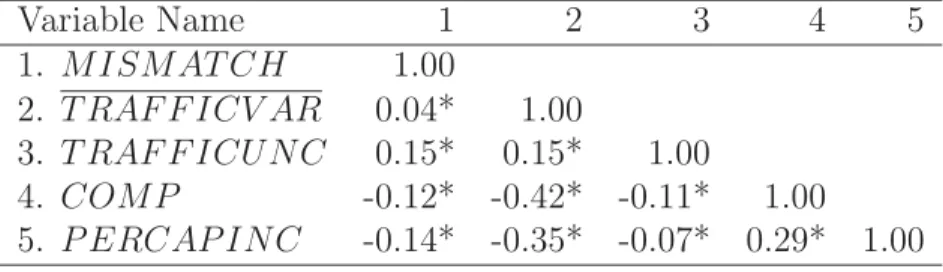
3.3 Correlations among longitudinal variables . . . 84

3.4 Correlations among cross-sectional variables . . . 85

3.5 Summary Statistics for Store Related Variables for Diﬀerent Time Slots Within a Weekday . . . 86

3.6 Summary Statistics for Store Related Variables for Diﬀerent Time Slots Within a Weekend . . . 87

3.7 Summary Statistics for Store Related Variables for Diﬀerent Days (Monday-Sunday) . . . 88

3.8 Summary Statistics for Store Related Variables for Diﬀerent Months (January-June) . . . 89

(10)

3.10 Independent-Samples T-Tests for Comparison of Non-Holidays (G1)

ver-sus Holidays (G2) . . . 91

3.11 Regression Results of First Stage Equations . . . 92

3.12 Regression Results of Second Stage Equation . . . 93

3.13 Regression Results for the Labor Mismatches Equation . . . 93

3.14 Summary of Hypotheses and Results . . . 93

3.15 Sensitivity Analysis for H2 for diﬀerent Traﬃc Uncertainty Models . . . 94

3.16 Sensitivity Analysis for H4 for diﬀerent Traﬃc Uncertainty Models . . . 95

3.17 Sensitivity Analysis for H4 for diﬀerent Mismatch Models . . . 95

3.18 Sensitivity Analysis for H1 and H2 . . . 96

A1 Notation. . . 147

A2 Scenarios examined. . . 148

A3 Full Factorial Design 1. . . 149

A4 Full Factorial Design 2. . . 149

A5 Expressions for scenario N ISS. . . . 152

A6 Impact of competition on retailer 1 in scenario N ISS. . . . 153

A7 Expressions for scenario INSS. . . 154

A8 Impact of competition on retailer 1 for scenario INSS. . . 155

A9 Expressions for scenario N IN S. . . . 163

A10 Impact of competition on retailer 1 for scenario N IN S. . . . 164

A11 Expressions for scenario IN N S. . . . 168

(11)

LIST OF FIGURES

2.1 Consumer valuation before and after the investment. . . 17

2.2 Duopoly. . . 19

2.3 Retailer 1’s proﬁt versus mean shift in scenario NISS. . . 31

2.4 The impact on retailer 1’s proﬁt based on the analytical results in sce-nario INSS. . . 34

2.5 Impact of competition in a low proximity and low market regime. . . . 36

3.1 A Framework for Analyzing Store Performance . . . 54

3.2 Factors Inﬂuencing Store Performance . . . 55

3.3 Correlation between conversion rate and basket value for one store . . . 79

3.4 Correlation between average conversion rate and average basket value across stores . . . 80

3.5 Correlation between conversion rate and intra-day traﬃc variability for one of the stores . . . 80

3.6 Correlation between basket value and traﬃc uncertainty across stores . 81

3.7 Correlation between average traﬃc uncertainty and average store traﬃc across stores . . . 81

4.1 Scenario Dominance for a Monopolist Under Stochastic Demand and Diﬀerent Investment Costs . . . 111

4.2 Scenario Dominance (obtained analytically) for a Symmetric Duopolist Under Deterministic Demand and Diﬀerent Investment Costs . . . 120

(12)

4.4 Scenario Dominance for a Symmetric Duopolist Under Stochastic De-mand and Equal Investment Costs . . . 129

4.5 Scenario Dominance (obtained analytically) for a Symmetric Duopolist Under Stochastic Demand and Diﬀerent Investment Costs . . . 132

4.6 Scenario Dominance (obtained numerically) for a Symmetric Duopolist Under Stochastic Demand and Diﬀerent Investment Costs . . . 133

A1 The impact on retailer 1’s proﬁt based on the analytical results in sce-nario NINS. . . 161

A2 The impact on retailer 1’s proﬁt based on the analytical results in sce-nario INNS. . . 165

(13)

CHAPTER 1 Introduction

1.1 Research Motivation

The retail industry is one of the most dynamic and inﬂuential industries in developed

economies. In the U.S. the retail business represents about 40% of the Gross

Do-mestic Product (GDP) and is the largest employer (Fisher and Raman (2001)). The

intensiﬁed competition that the retail industry faces with the emergence of increasing

numbers of new players in both the local and global markets has forced retailers to

critically examine and redesign both their operations and marketing strategies. To

re-main competitive, many retailers have diﬀerentiated themselves by designing enhanced

customer experiences and other strategies to distinguish themselves from competition.

Such practices have provided a fertile ground and new contexts for research in the

re-tail operations arena. This dissertation comprising of three essays aims to shed light

to some important aspects of retail operations that have emerged due to the current

practices. The aim of this research is to develop theoretical insights to help retailers

understand their store performance and eﬀectively manage strategies geared towards

enhancing demand and consumer valuation about their product oﬀerings. In Chapter 2

we examine investments in technologies that can aﬀect consumer valuation and focus on

(14)

Chapter 3 we study the impact of labor and traﬃc characteristics on store performance

using proprietary data of a retail chain. In Chapter 4 we focus on general services

that retailers could provide to enhance demand and examine their temporal

manage-ment under competition in the face of demand uncertainty. Chapter 5 concludes the

dissertation. A brief overview of each chapter of the dissertation follows.

1.2 Dissertation Overview

1.2.1

Chapter 2

With increased competition in the retail industry many retailers such as Best Buy are

investing in technology, employee training, and presentation in order to improve

con-sumers’ valuation of their product oﬀerings. Such investments in pre-purchase activities

to enhance consumer valuation are costly and are designed to increase the possibility

of purchase, but they do not lead to “stickiness”. In particular, increases in consumer

valuation through pre-purchase services are prone to free-riding since consumers receive

the beneﬁts of such activities oﬀered by a retailer, but may decide to purchase a

prod-uct at another retailer. Gateway’s Country Stores and their subsequent demise provide

a characteristic example of the free riding problems (Frei (2006)).

Chapter 2 investigates the factors that retailers should consider before investing

in pre-purchase activities in order to increase consumer valuation and examines their

effect on retailers’ pricing and profits. We develop a stylized model using first

princi-ples on the distribution of consumer valuation and study a duopoly in which retailers

compete on the basis of price and consumer search is allowed between the two retailers.

In such a setting, a retailer may make investments to increase consumer valuation for

his product, but the ﬁnal sale could be made at the other retailer, who did not invest

(15)

investment and pricing through a computational study. Then we focus on the pricing

game only and establish the pricing Nash equilibria. We characterize the competitive

eﬀects under diﬀerent regimes related to market expansion, retailers’ physical

proxim-ity, direction of consumer ﬂow, and magnitude of change in consumer valuation for

two asymmetric investment structures. Next, we focus on a special case in which the

competing retailers are symmetric and characterize the possible Nash equilibria

invest-ment strategies depending on the investinvest-ment cost. Finally, we present a model with an

endogenous level of investment and analyze the symmetric equilibrium for a symmetric

duopoly.

Our main results are as follows. When the investment decision is endogenous, we

establish the surprising result that in the majority of instances both retailers will decide

to invest in equilibrium but price the product in a manner to avoid consumer search

between them. We also ﬁnd that the proximity of retailers has an interesting

non-monotonic impact on their decisions to invest. Retailers tend to invest in technology

when they are either very close or very far away but refrain from investing in the

in-termediate range. When we further focus only on the pricing game, we ﬁnd two major

eﬀects related to improvements in consumer valuation. First, consistent with popular

belief, we ﬁnd that there is a threshold eﬀect whereby a retailer could overcome

com-petitive eﬀects by improving consumer valuation. However, there are situations where

a greater improvement in consumer valuation by a retailer could lead to lower proﬁts.

Second, we ﬁnd evidence for a free-riding eﬀect where a retailer who does not invest

in valuation enhancement practices could beneﬁt from an innovative competitor who

increases consumer valuation beyond a threshold. When we focus on symmetric

retail-ers we ﬁnd that as the investment cost increases the Nash equilibrium strategies shift

from both retailers investing, to only one retailer investing (either retailer 1 or retailer

(16)

of investment is endogenous, we show that a symmetric duopolist’s optimal strategy to

cover his whole local market or part of his market depends on the eﬀectiveness of his

investment cost and the optimal price may indeed decrease with the per unit cost of

acquiring the product.

1.2.2

Chapter 3

The intensiﬁed competition in the retail industry has forced retailers to place enormous

importance on store performance metrics. Several retailers nowadays track two metrics

conversion rate, the percentage of incoming traﬃc who purchased, and basket value,

the average dollar amount spent by customers. Both metrics are important indicators

of store performance. Conversion rate, for example, has been found to be strongly

correlated with customer loyalty while basket value, on the other hand, is typically

linked to the proﬁtability of the retailer. Both conversion rate and basket value can

be correlated with traﬃc characteristics due to many factors including labor, consumer

purchase behavior, economic conditions, product availability, and merchandise

assort-ment.

In Chapter 3, we use proprietary data pertaining to a retail chain to conduct a

descriptive study of conversion rate and basket value. Speciﬁcally, we consider the

correlation between store performance and intra-day traﬃc variability and traﬃc

un-certainty. We also measure traﬃc-labor mismatches and study if they explain the

observed correlations in our sample.

The results of our study are as follows: First, we report the within-store results.

We ﬁnd that intra-day traﬃc variability is negatively correlated with both conversion

rate and basket value. A 1% increase in traﬃc variability is associated with a 0.094%

decrease in conversion rate in a store and 0.037% decrease in basket value. We also ﬁnd

(17)

an increase in store labor at a diminishing rate. A 1% increase in labor is associated

with a 0.102% increase in conversion rate and 0.066% increase in basket value. In

addition, we ﬁnd that conversion rates are higher during holidays but basket values are

lower suggesting that price promotions oﬀered during the holiday season cause more

customers to purchase but do not lead to higher levels of purchasing. Moreover, we

ﬁnd that both conversion rates and basket values exhibit signiﬁcant seasonality.

Next, we report the across-store results. We ﬁnd that stores with higher traﬃc

uncertainty have lower conversion rates but similar basket values. We also ﬁnd that

stores that have higher traﬃc variability and higher traﬃc uncertainty have higher

mismatches between required labor and actual labor. Furthermore, our tests reveal

that stores that have lower foot-traﬃc have higher traﬃc uncertainty, resulting in

mis-matches between required labor and actual labor. A surprising result of our analysis is

that competition as measured here does not aﬀect conversion rates and basket values.

Finally, we ﬁnd that stores located in neighborhoods with higher per capita income

have higher conversion rates but similar basket values.

1.2.3

Chapter 4

In Chapter 4 we focus on understanding the temporal management of investments in

activities that can enhance demand under competition in the face of demand

uncer-tainty. In many settings, retailer investments in experience activities are important

in inﬂuencing demand for a product. For example, a retailer can stimulate demand

through various ways such as provide training to its sales personnel to promote a given

product, create special areas to show case a product or even invest in technology that

oﬀers a unique experience for a product. All the above activities which we will be

referring to as “service” can aﬀect the purchasing decision of customers. The planning

(18)

launched in a market. In the case of new product introduction, the retailer needs not

only to decide the optimal price and service investments for the product but also when

to invest in such experience activities. Given that market demand could be highly

uncertain, a retailer may choose to wait until he receives some information regarding

the market state before investing in such activities or he may want to make all these

investments upfront to take advantage of possible reduced investment costs.

In this chapter we develop a two-stage model in order to examine two alternatives

that retailers typically have in terms of timing their investments under both monopoly

and symmetric duopoly settings. The ﬁrst alternative is to invest in service in advance

of the selling season without knowing the market state (i.e., invest in the ﬁrst stage) and

the second alternative is to invest in service after the market state realizes (i.e., invest in

the second stage). In both cases a retailer decides on pricing after observing the demand

(i.e., in the second stage). For the monopoly we further examine a hybrid strategy in

which a retailer can invest both before and after the demand state is known. Typically,

investing after the demand state is known is associated with higher investment costs.

We analyze these settings under both equal and diﬀerent investment costs across stages.

In addition, we investigate the deterministic demand case for the symmetric duopoly

and contrast our results with the stochastic demand case. In the case of a deterministic

demand these alternatives translate to making sequential decisions (i.e., ﬁrst service

and then price) as opposed to simultaneous decisions (both service and price).

Our major ﬁndings in Chapter 4 are as follows. For a monopolist who faces

stochas-tic demand and incurs diﬀerent investment costs across stages, we show that a hybrid

strategy always dominates a strategy in which a retailer invests only before or only

after the market state is known. In addition, we show that a monopolist would prefer

to delay investments until demand is realized only when the market variability is high

(19)

mo-nopolist would prefer to invest before the demand is realized. This result is in contrast

to the case of equal investment costs in which a monopolist would always defer such

investments until after the demand is realized.

For a symmetric duopolist who faces deterministic demand and incurs the same

investments costs across stages we show that the dominant strategy is always to make

service investments in the ﬁrst stage. We ﬁnd that this is not always the case when

the duopolist incurs higher investment costs in the second stage. Interestingly, when

the intensity of competition of service is high, a symmetric duopolist could be better

oﬀ to invest in the second stage as the diﬀerential cost of investment in the two stages

increases. We also ﬁnd computationally that the equilibrium strategies for a symmetric

retailer can shift in a non-monotonic fashion as the diﬀerential cost of investment in

the two stages increases. In particular, a retailer could invest in the ﬁrst stage for high

and low diﬀerential costs and in the second stage for intermediate values of diﬀerential

costs.

For a symmetric duopolist who faces stochastic demand and incurs same costs across

stages, the dominant strategy is to invest in demand enhancing activities in the ﬁrst

stage in all regimes except for one characterized by high demand variability, low

in-tensity of competition in service, and high investment cost. This result shows that the

competitive dynamics could signiﬁcantly diminish the value of delaying investments

af-ter demand is realized. We further characaf-terize some of the investment strategies when

a duopolist incurs higher investment costs in the second stage. Interestingly, we ﬁnd

that in the case of high intensity of service competition increase in demand variability

could make investing more preferable in the ﬁrst stage than in the second stage if the

(20)

CHAPTER 2 Improving Valuation Under

Consumer Search:Implications for

Pricing and Proﬁts

2.1 Introduction

The retail sector is a vital sector in most modern economies. In the U.S. for example,

the retail industry represents about 40% of the economy and is the largest employer

(Fisher and Raman (2001)). As a result, several researchers have examined diﬀerent

retail operations issues, which include inventory management and store execution (see

Eppen and Iyer (1997), Tsay and Agrawal (2000), Raman et al. (2001), Fisher et al.

(2006), Nagarajan and Rajagopalan (2008) for representative work).

With increased competition, retailers are trying to identify ways to diﬀerentiate

themselves. One strategy has been to invest in practices that increase consumer

valua-tion of their product oﬀerings. Our interacvalua-tions with a former top executive at Magnolia

Home theater stores, specialized stores at Best Buy geared towards high end electronic

(21)

em-ploy to improve consumer valuation of their product oﬀerings (Freeland (2007)). These

practices include improving the ambience of the store to enhance the presentation of

the product category as well as hiring well-trained experts as salespeople to explain

the product characteristics. Investments in strategies to increase consumer valuation

entail some risk because they are usually costly and may not pay oﬀ in increased sales.

Another risk is that a retailer may invest in an enhanced presentation to sell a

prod-uct, but the customer decides to purchase it at another retailer, who hasn’t made the

investment - leading to the free-riding phenomenon. Gateway’s country stores

pro-vides an example of free riding. As indicated by Frei (2006), “When Gateway’s new

stores opened in 1996, they were undeniably impressive. Employees were experienced,

helpful, and abundant (the employee-to-customer ratio was unusually high). Excellent

educational materials were on hand, and the stores were conveniently located to ensure

heavy foot traﬃc. Unfortunately, Gateway hadn’t guaranteed that the people receiving

the beneﬁts of all that pre-purchase accommodation would also bear the costs. Far too

often, customers took their newly acquired understanding of what they needed and

how the product worked and then placed an order with one of Gateway’s low-price

competitors”.

These observations suggest that in addition to managing inventory in stores (which

often is the focus of studies in operations management) there are other aspects of

store operations that determine eventual sales. Our work studies retailer initiated

increases in consumer valuation, which could aﬀect consumers’ purchasing decision and

(22)

consumer valuations that are experiential i.e., remain with the consumer even when

they go to another retailer. We do not consider retailer-speciﬁc (“sticky”) increases in

consumer valuations such as after-purchase services and coupon oﬀerings which are not

prone to free riding. Speciﬁcally, we are interested in addressing the following questions:

How do market characteristics aﬀect the retailer’s decision to invest in such practices?

How does the ability of a retailer to change consumer valuation for a product aﬀect his

retail price and proﬁt under competition? These questions address issues that retailers

need to be aware of when they engage in consumer valuation enhancement activities.

To answer these questions, we ﬁrst develop a stylized model using ﬁrst principles

on the distribution of consumer valuation. We assume that consumer valuation is

uni-formly distributed and an improvement is captured by a right shift of the distribution.

We consider a two-stage game in a duopoly setting, where consumers could search

among two retailers who oﬀer a single product. In the ﬁrst stage, the retailers decide

whether to invest in improvements in customer valuation. In the second stage, given

the investment decisions in the ﬁrst stage, the retailers engage in price competition. We

explore the Nash equilibria in terms of both investment and pricing through a

compu-tational study. Then we focus on the pricing game only and establish the pricing Nash

equilibria. We characterize the competitive eﬀects under diﬀerent regimes related to

market expansion, retailers’ physical proximity, direction of consumer ﬂow, and

magni-tude of change in consumer valuation for two asymmetric investment structures. Next,

we focus on a special case in which the competing retailers are symmetric and

(23)

cost. Finally, we present a model with an endogenous level of investment and analyze

the symmetric equilibrium for a symmetric duopoly.

Our main results are as follows. When the investment decision is endogenous, in

the majority of instances both retailers decide to invest in equilibrium but they price

the product in a manner to avoid consumer search between them. We also ﬁnd that

the proximity of retailers has an interesting non monotonic impact on their decisions

to invest in that retailers tend to invest when they are very close or very far away but

refrain from investing in the intermediate range. When we further focus on only the

pricing game we ﬁnd two major eﬀects related to improvements in consumer valuation.

First, consistent with popular belief, we ﬁnd that a retailer could overcome competitive

eﬀects by improving consumer valuation beyond a certain threshold. However, there

are situations where a greater improvement in consumer valuation by a retailer could

lead to lower proﬁts. Second, we ﬁnd evidence of free-riding, where a retailer who

does not invest could beneﬁt from an innovative competitor who increases consumer

valuation beyond a threshold. When we focus on symmetric retailers we ﬁnd that as

the investment cost increases, the Nash equilibrium strategies shift from both retailers

investing, to only one retailer investing (either retailer 1 or retailer 2), and ﬁnally to

neither retailer investing. Finally, for the extension where the level of investment is

endogenous, we show that a symmetric duopolist’s optimal strategy to cover his whole

local market or part of his market depends on his investment cost eﬀectiveness and the

optimal price charged by him may indeed decrease with the per unit cost of acquiring

(24)

The rest of the chapter is organized as follows. Section 2 brieﬂy reviews the relevant

literature. In Section 3, we describe the two-stage game for the duopoly and provide

insights on the retailers’ investment decisions. Section 4 focuses on the pricing game.

Section 5 examines a special case in which both retailers are symmetric. In Section 6,

we present an extension to the basic model. Finally, we conclude by summarizing our

ﬁndings and provide future research directions in Section 7. We present a summary of

our mathematical notation in Appendix A. Proofs of all the results are in Appendix.

2.2 Literature Review

Our work relates to the retail price competition literature that has been extensively

studied by research in economics, marketing, as well as operations management. Initial

works in this stream focused on competition among brick-and-mortar retailers. In

addition to price competition among traditional retailers, there has recently been a

number of papers that focus on pricing in diﬀerent contexts such as multi-channel

supply chains and e-commerce. Cattani et al. (2004) and Tsay and Agrawal (2004)

provide extensive reviews of this literature.

There have also been works under retail competition that have incorporated a

“ser-vice” component as a decision variable for retailers in addition to pricing. Two diﬀerent

types of service are found in the literature: (i) service experience which can be

con-sumed by the customer without necessarily making a purchase at the retailer who oﬀers

(25)

de-rived by making a purchase at the retailer who oﬀers it (e.g., generous warranties,

free-delivery, and installation).

Our work is related to the stream of literature that considers the ﬁrst type of

service. In settings where the pre-sale activities are conducted independently from the

actual sale of the product, the riding problem occurs. The main focus of the

free-riding literature has been the negative impact of free free-riding on the retailers’ incentive

to provide costly pre-sale service and the way that retailers and manufacturers could

prevent free riding (see Carlton and Perloﬀ (2000), Carlton and Chevalier (2001)).

From this literature the papers by Bernstein et al. (2006) and Shin (2007) are related

to our work.

Bernstein et al. (2006) also explore the idea that consumer valuation could be

in-creased by making appropriate investments. These authors consider

manufacturer-retailer competition and are interested in how free-riding aﬀects a manufacturer’s

de-cision to open a direct store. In contrast, we focus on retailer competition and are

interested in understanding - (1) how the market characteristics, customer search

be-havior, and magnitude of change in consumer valuation could aﬀect retailers’ investment

decisions; (2) how free-riding and proﬁt-loss to competition are aﬀected by the above

factors. Bernstein et al. (2006) ﬁnd that the direct store price is always higher than

the retail price as long as visiting the direct store increases consumer valuation. Our

computational study, on the other hand, shows cases where the retailer who invests to

increase consumer valuation but has a smaller market share could oﬀer a lower price

(26)

proportion of searching consumers is high.

Shin (2007) considers two retailers selling the same product competing for the same

customers who are heterogenous in terms of their opportunity costs for shopping and

can be of two types: informed and uninformed. The author focuses on sales assistance

that resolves the matching uncertainty between the retailers’ product speciﬁcation and

consumers’ needs. In our work, we also consider two retailers selling the same product

but competing for customers who are heterogenous in terms of their valuation for the

retailers’ product. We focus on retailers’ investments which can increase customer

valuation of their product and model explicitly the impact of such investments on the

consumers’ valuation distribution.

Our work contributes to the existing literature in the following aspects. First, we

develop a model that allows us to study the impact of increasing consumer valuation.

Second, we provide managerial insights on how the market characteristics and

con-sumer search behavior could impact the retailers’ investment strategies. Third, we

provide insights on how the ability of retailers to inﬂuence consumer valuation impacts

competitive and free riding eﬀects under diﬀerent regimes related to market expansion,

retailers’ physical proximity, consumer search behavior, and magnitude of changes in

(27)

2.3 Model

This section is organized as follows. In §2.3.1 we present a model of how consumer

valuation increases. Then, in §2.3.2 we present our duopoly setting and describe the

consumer search behavior. In §2.3.3 we describe the two-stage investment and pricing

model. Finally, we provide some computational insights in §2.3.4.

2.3.1 Modeling of Consumer Valuation Increase

We first consider a risk neutral firm (retailer 1) which offers one product in a market of

population size μ. Consumers are heterogeneous in the valuation of the product. We

denote the consumption value (alternatively called “willingness to pay”) by V which

is assumed to be uniformly distributed (across the population of consumers) between

0 and 1. The retailer oﬀers the product at price p₁ and incurs cost per unit c₁ for

acquiring the product. Consumers who visit the retailer incur a cost k₁. “This cost

can include the opportunity cost of time, the real cost of travel, and the implicit cost

of inconvenience” (Balasubramanian (1998)). We will be referring to k₁ as traveling

cost. Therefore, consumers whose valuation is greater than or equal to the sum of

retail price p₁ and cost k₁ (p₁+k₁) buy the product from retailer 1. In that case, the

retailer’s expected demand and proﬁt are qN

1 =μP(V ≥p1+k1) =μ(1−p1−k1) and

πN₁ = (p₁−c₁)q₁N (superscript N refers to the scenario in which the retailer does not invest to increase consumer valuation). We provide a summary of all the scenarios in

(28)

to his retail price. The resulting optimal price, demand, and proﬁt arep∗N

1 = 1+

c1−k1 2 ,

q∗N

1 = (1−

c1−k1)μ

2 , and π∗

N

1 = (1−

c1−k1)2μ

4 , where 0≤c1+k1 ≤1.

If the retailer engages in consumer-valuation-enhancing activities, a consumer whose

valuation was v prior to visiting the retailer enjoys a valuation ˆv after visiting the

retailer. In the basic model, we assume that the investment leads to a ﬁxed linear

shift α (i.e., ˆV will be uniformly distributed between α and 1 +α as illustrated in

Figure 1). In order to accomplish these activities, we assume that the retailer incurs

a ﬁxed cost I₁. This assumption represents situations where ﬁxed investments lead to

a given increase in consumer valuation1. Note that a shift in the consumer valuation

distribution leads to an increase in the average consumer willingness to pay for the

product. As a result, for a pricep₁ the demand before investment isqN

1 =μ(1−p1−k1)

while the demand after investment isq₁I =μP( ˆV ≥p₁+k₁) =μ(1+α−p₁−k₁), which is identical to the demand expression obtained when oﬀering a price discount ofαper unit.

Hence, a linear shift model of consumer valuation may seem similar to a price discount

model. However, there are critical diﬀerences. First, a linear shift model of consumer

valuation and a price discount model2 _{lead to diﬀerent proﬁt functions which will result}

in diﬀerent optimal pricing, demands, and proﬁts. Second, and more importantly, a

price discount creates loyalty to the retailer who runs the promotion whereas increasing

consumer valuation for a product does not guarantee that the consumer would make

the purchase from the retailer who exerts such eﬀorts.

1_{We study an extension of this basic model in Section 6 in which}_α_{is endogenous and the investment}

cost is dependent onα.

2_{In a price discount model the proﬁt function is}_π₁_{= (}_p₁₋_α₋_c₁₎_μ_{(1 +}_α₋_p₁₋_k₁_{) whereas in}

(29)

Before Investment

Probability of buying

0 1

After Investment ݌ଵ൅ ݇ଵ

ܽ ͳ ൅ ܽ

݌ଵ൅ ݇ଵ

Probability of buying

FIGURE 2.1: Consumer valuation before and after the investment.

The objective for the retailer is to maximize his expected proﬁt πI₁ = (p₁ −c₁)q₁I -I₁, by deciding on the price under the constraint that α ≤ p₁ +k₁ ≤ 1 +α. The

optimal price, demand, and proﬁt as functions of the mean shiftαare p∗I

1 = 1+

α+c1−k₁

2 ,

q₁∗I = (1+α−c₂1−k1)μ, and π∗₁I = (1+α−c₄1−k1)2μ−I₁, where 0≤α ≤1 +c₁ +k₁.

2.3.2 Duopoly and Search

We now consider two retailers in the market (retailer 1 and retailer 2) who oﬀer the

same product at prices p₁ and p₂ and incur per unit costs of acquiring the product c₁

and c₂ respectively. Such diﬀerences in retailers’ costs may be a reﬂection of buying

power as well as their operational performance. Both retailers can invest to increase

consumer valuation by incurring investment costsI₁andI₂. We assume that the change

in consumer valuation is identical for both retailers but the investment costs of the two

retailers are diﬀerent to allow for heterogeneity in the retailers’ investment eﬀectiveness.

We further assume that the two retailers are located at some distance from each other

and that the introduction of retailer 2 may bring additional people in to the market

(30)

expansion in the market and denote by the additional people in the market (i.e., the

new market size will be μ+, where ≥0).

We assume that γ proportion of the total population is located near retailer 1 and

as a result this proportion visits retailer 1 ﬁrst. The remaining (1-γ) visits retailer

2 ﬁrst. Consumers who visit retailer 1 and retailer 2 incur traveling costs k₁ and k₂

respectively. The search occurs as follows (see Figure 2.2). A consumer visits her local

retailer ﬁrst. She buys the product from that retailer provided that she obtains

non-negative consumer surplus i.e.,v ≥pi+ki. If the consumer surplus is negative she does

not buy the product at her local retailer. A fraction of such consumers δ (0≤ δ ≤ 1)

who have visited their local retailer and have not obtained positive consumer surplus

would be willing to search with updated consumer valuation the other retailer before

leaving the system. The cost that a consumer incurs traveling from one retailer to the

other is denoted by Δk. Similar to Lal and Sarvary (1999), when consumers visit their

local retaileriﬁrst they incur a traveling costkiassociated with the cost of undertaking

the shopping trip, and when consumers go from one retailer to the other, they incur a

traveling cost Δk of visiting an additional retailer. Note that we are not modeling the

case where a consumer visits the other retailer after having visited her local retailer,

seeking price-matching guarantee refunds. Though price matching is common in the

retail industry, research shows that on average only about 5 to 7.4 percent of consumers

seek price matching guarantee refunds (Moorthy and Winter (2004), Kukar-Kinney

(2005)). We also do not consider the situation where, after visiting the second store

(31)

RETAILER 1

cost per unit ܿଵ consumer traveling cost ݇ଵ

cost of Investment ܫଵ

RETAILER 2

cost per unit ܿଶ consumer traveling cost ݇ଶ

ଶ cost of Investment ܫ Traveling cost

from one retailer to the other ο݇

ߜ

Retail price ݌ଵ ߛ ͳ െ ߛ Retail price ݌ଶ

POTENTIAL CUSTOMERS

ሺߤ ൅ ߝ)

FIGURE 2.2: Duopoly.

reasonable assumption when the price diﬀerential between the stores is not signiﬁcant.

Our search scheme is close to that of Anupindi and Bassok (1999) and Ahn et al.

(2002). In Anupindi and Bassok (1999) consumers buy the product from their local

retailer. In the event of a stock-out a fraction of the unsatisﬁed customers looks for

the product at another retailer. Since we assume that the demand is deterministic so

there is no stock-out, consumers buy the product from their local retailer provided that

they obtain positive consumer surplus. A fraction of consumers who have visited their

local retailer and have not obtained positive consumer surplus will continue their search

with updated consumer valuation. In Ahn et al. (2002) a manufacturer-owned store

(outlet) and an independent retail store are located in diﬀerent markets. Each consumer

makes the initial attempt to purchase at the store that is closer. All consumers who

have visited the independent retail store and did not obtain positive consumer surplus

travel to the manufacturer-owned store (i.e., one way movement of consumers). Our

(32)

incur a cost when they visit their local retailer (in their case such cost is zero), (ii)

consumers can search both retailers (in their case there is one way ﬂow) and (iii) only a

proportion of consumers who encounters non-positive consumer surplus searches both

retailers, while the rest leave the system without making a purchase (in their case this

proportion is one). In addition, our work is diﬀerentiated from the above search related

literature in the incorporation of updated consumer valuations.

2.3.3 Investment Pricing Game

We consider two retailers engaging in an investment pricing game with the following

sequence of events.

1. The retailers simultaneously decide whether to invest in improvements in

cus-tomer valuation.

2. Based on their investment decision in event 1, the retailers simultaneously

deter-mine their prices.

The above events constitute a two-stage game. In the ﬁrst stage the retailers make

investment decisions to improve customer valuation. These decisions can lead to the

following possible investment scenarios.

(i) Neither retailer invests (denoted as (NI,NI)).

(ii) Retailer 1 does not invest but retailer 2 invests (denoted as (NI,I)).

(iii) Retailer 1 invests but retailer 2 does not invest (denoted as (I,NI)).

(iv) Both retailers invest (denoted as (I,I)).

(33)

retailers decide on their prices. Let xi ∈ {0,1} denote retailer i’s decision to invest or

not in improving customer valuation. Then, retailer i’s problem in stage 1 is given by

max

xi∈{0,1}

πi(xi, xj, pi, pj) = (pi−ci)qi(xi, xj, pi, pj)−xiIi

where

qi(xi, xj, pi, pj) = (μ+)γ(xi(1 +α−pi−ki) + (1−xi)(1−pi−ki))

+ (1−γ)δ(μ+)(1−xi)(1−xj)(pj −pi−Δk)+

+ (1−γ)δ(μ+)(1−xi)xj(pj −pi−Δk)+

+ (1−γ)δ(μ+)xi(1−xj)(pj +α−pi−Δk)+

+ (1−γ)δ(μ+)xixj(pj−pi−Δk)+

The ﬁrst term of the demand expression (i.e., (μ+)γxi(1 +α−pi −ki)) denotes

the demand from local consumers if retailer i invests. The second term (i.e., (μ+

)γ(1−xi)(1 −pi −ki)) denotes the demand from local consumers if retailer i does

not invest. The remaining terms of the demand expression denote the demand from

searching consumers for the above four possible investment strategies (i)-(iv) chosen by

the retailers respectively.

We use backwards induction to solve this two stage-game. For each investment

scenario ((i)-(iv)) we need to solve the second-stage problem and identify the pricing

(34)

we distinguish four theoretically possible cases (because of the (·)+ _{operator) that}

correspond to the following four possible consumer search schemes depending on the

retailers’ prices:

(1) Consumers do not search (denoted as (NS,NS)).

(2) Consumers search from retailer 2 to retailer 1 (denoted as (NS,S)).

(3) Consumers search from retailer 1 to retailer 2 (denoted as (S,NS)).

(4) Consumers search both retailers (denoted as (S,S)).

Speciﬁcally, for investment scenarios (ii) and (iii) we need to consider all four cases

(1)-(4) in the second stage whereas for investment scenarios (i) and (iv) we only need

to consider cases (1)-(3) as shown in Proposition 1. All proofs are in Appendix.

Proposition 1 In investment scenarios (ii) and (iii) both retailers can obtain sales

from the consumers who search between retailers. In investment scenarios (i) and (iv)

only one retailer can obtain sales from the consumers who search.

Hence, there are 14 possible cases in the second stage of the game that need to be

analyzed. However, we can indeed show that for a given combination of investment

and consumer search scheme, there exists a unique equilibrium in the pricing game.

Proposition 2 In the two-retailer pricing game a unique Nash equilibrium exists for

every combination of investment scenario and consumer search scheme.

Deriving the two-stage game Nash equilibrium (x∗_i, x∗_j, p∗_i, p∗_j) for an arbitrary set of parameters is analytically intractable. Therefore, we ﬁrst explore the Nash equilibria

(35)

effects of changing different parameters such as γ, δ, Δk, and different types of costs

on the Nash equilibria. Then, in the following section, we focus on the pricing game

only and theoretically characterize the pricing Nash equilibria for a given investment

scenario and consumer search scheme.

2.3.4 Computational Insights

We now describe our computational study and some of the interesting insights that we

obtained for the pricing and investment game. We used a full factorial design

experi-ment summarized in Table A3 in Appendix. We identify the Nash equilibria in terms of

the investment decisions of the two retailers in the two-stage game as follows: We start

backwards to solve the second stage of the game ﬁrst. For each of the four possible

investment scenarios ((i)-(iv)), we compute the pricing Nash equilibria of the retailers

assuming a given consumer search scheme ((1)-(4)). For each instance of a given

in-vestment scenario, we identify the consumer search scheme that is a Nash equilibrium

(i.e., the consumer search scheme that is being induced by the Nash equilibrium pricing

strategy of the retailers for a given investment scenario). We refer to this consumer

search scheme as search Nash equilibrium. During our computational study, we found

that there are instances that lead to two search Nash equilibria that cannot be ranked

because one retailer is better oﬀ with one consumer search scheme and the other retailer

is better oﬀ with the other search scheme. We did not consider such instances in the

ﬁrst stage of the game where the retailers make a decision on whether to invest or not.

(36)

second stage of the game, we can identify the Nash equilibrium investment strategy for

the retailers.

Tables 2.1 and 2.2 provide a summary on the types of Nash equilibria investment

strategies as well as the Nash equilibria search strategies which result from the retailers’

pricing decisions. Table 2.3 summarizes the frequency of occurrence in our experimental

setup of each consumer search scheme for a given investment equilibrium scenario.

TABLE 2.1: Characterization of investment Nash equilibria.

Type of strategies (NI,NI) (NI,I) (I,NI) (I,I) Two Nash equilibria

% 16.143% 22.125% 27.697% 33.16% 0.874%

TABLE 2.2: Characterization of search Nash equilibria.

Type of strategies (NS,NS) (NS,S) (S,NS) (S,S) Two Nash equilibria

% 30.948% 27.752% 25.239% 15.187% 0.874%

TABLE 2.3: Investment and Search Nash equilibria.

(NS,NS) (NS,S) (S,NS) (S,S)

(NI,NI) 57.699% 23.012% 19.289% NA

(NI,I) 8.519% 40.37% 22.716% 28.395% (I,NI) 13.609% 20.513% 33.728% 32.15%

(I,I) 48.188% 28.418% 23.394% NA

Here are some interesting observations with respect to the impact of the retailers’

investments on the consumer search scheme.

(1) We notice that the most prevalent Nash equilibrium investment strategy

cor-responds to both retailers investing. There is a very small proportion of instances

(0.874%) that lead to two pure investment Nash equilibria (see Table 2.1).

Interest-ingly, the majority of instances lead to retailers pricing in such a manner so that there

(37)

(2) When both or none of the retailers invest, then they price in such a manner

so as to discourage consumer search. Speciﬁcally, 48.188% and 57.699% of situations

where the resulting Nash equilibria is such that both retailers invest or neither retailer

invests, respectively, lead to no search between the retailers. This result is interesting

particularly in the case of both investing, because it enables the retailers to avoid price

competition due to search.

(3) In a number of cases, consumers may decide to search a retailer who invests.

For example, Table 2.3 shows that 20.513% of the cases where retailer 1 invests lead to

consumers searching that retailer and 22.716% of the cases where retailer 2 invests lead

to consumers searching that retailer. In those cases, it is quite possible that the retailer

who has made the investment decides to price lower than the other retailer, and this

eﬀect is more profound when the percentage of consumers willing to search increases.

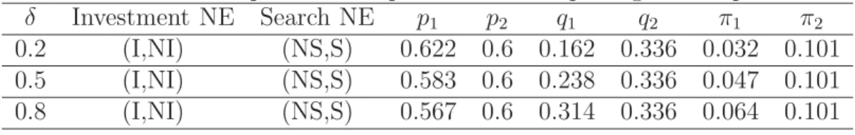
Such an example is illustrated in Table 2.4 with parameter values γ = 0.2, = 0.4,

μ = 1, c₁ = c₂ = 0.3, k₁ = k₂ = 0.1, Δk = 0.05, I₁ = 0.02, I₂ = 0.1, and α = 0.2.

Since I₁ << I₂ only retailer 1 has an incentive to invest. Note that retailer 1 is at a

disadvantage in terms of market share since γ = 0.2. At low values of δ, retailer 1’s

beneﬁt from consumers who search is low, thus, his incentive to attract consumers from

retailer 2 is low. Hence, retailer 1 prices higher than retailer 2. But as the proportion of

consumers who are willing to search increases, retailer 1’s beneﬁt from the consumers

who search is high. As a result, retailer 1 is willing to drop his price and prices lower

than retailer 2 (even though retailer 1 is the one who has invested).

(38)

TABLE 2.4: An example of the impact of δ on the pricing Nash equilibrium.

δ Investment NE Search NE p₁ p₂ q₁ q₂ π₁ π₂

0.2 (I,NI) (NS,S) 0.622 0.6 0.162 0.336 0.032 0.101

0.5 (I,NI) (NS,S) 0.583 0.6 0.238 0.336 0.047 0.101

0.8 (I,NI) (NS,S) 0.567 0.6 0.314 0.336 0.064 0.101

decisions of the retailers. Here are some of our key insights.

Eﬀect of Proximity: The proximity between the two retailers Δk has an

in-teresting non-monotonic behavior on the retailers’ investment decisions under certain

conditions. Speciﬁcally, we ﬁnd that at low and high values of Δk both retailers have

an incentive to invest, yet for intermediate values of Δk, only one of the retailers has

an incentive to invest. Table 2.5 illustrates such an example with parameter values

γ = 0.8, δ = 0.8, = 0.4, μ = 1, c₁ = c₂ = 0.4, k₁ = k₂ = 0.3, I₁ = I₂ = 0.02, and

α= 0.5.

TABLE 2.5: An example of the impact of Δk on the investment Nash equilibria.

Δk Investment NE Search NE p₁ p₂ q₁ q₂ π₁ π₂

0.02 (I,I) (S,NS) 0.8 0.64 0.448 0.282 0.159 0.048

0.1 (I,NI) (S,S) 0.778 0.542 0.509 0.177 0.173 0.034

0.2 (I,I) (NS,NS) 0.8 0.8 0.448 0.112 0.159 0.025

This can be explained because for low values of Δk, the retailers’ competition is very

intense which creates an incentive for both retailers to invest. For high values of Δk,

each retailer is actually acting as a monopolist who can make independent decisions

that do not have an impact on the other retailer. For the intermediate values of Δk, the

competition is not so intense and does not justify the retailer who is at a disadvantage

in terms of market share to commit to an investment decision. This insight suggests

(39)

could ignore the investments made by a retailer who is further away.

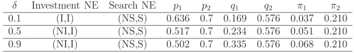
Eﬀect of Searching Consumers: In order to better understand the eﬀects of

the percentage of consumers willing to search δ, we considered three other values δ =

0.1,0.5,0.9 (see example in Table 2.6 with the following parameter values: γ = 0.2,

= 0.8, μ= 1, c₁ =c₂ = 0.3,k₁ =k₂ = 0.1, Δk = 0.05 , I₁ =I₂ = 0.02, and α= 0.2).

TABLE 2.6: An example of the impact of δ on the investment Nash equilibria.

δ Investment NE Search NE p₁ p₂ q₁ q₂ π₁ π₂

0.1 (I,I) (NS,S) 0.636 0.7 0.169 0.576 0.037 0.210

0.5 (NI,I) (NS,S) 0.517 0.7 0.234 0.576 0.051 0.210

0.9 (NI,I) (NS,S) 0.502 0.7 0.335 0.576 0.068 0.210

Note that in this case γ = 0.2, so retailer 1 is at a disadvantage with respect to the

market share, and hence, needs to price lower in order to attract more consumers. As

a result, consumers always search retailer 1 at equilibrium. Therefore, for low values

of search (δ) both retailers invest at equilibrium. But as the proportion of search

population (δ) increases, retailer 1 does not have an incentive to invest anymore and

is better oﬀ free-riding from retailer 2. Therefore, only retailer 2 invests at equilibrium

and consumers search from retailer 2 to retailer 1. We ﬁnd a similar symmetric eﬀect

when γ = 0.8 since retailer 2 is at a disadvantage in that case with respect to the

market share.

Eﬀect of Market Share, Total Market, and Costs: As expected, market share

γ plays a critical role in the retailer’s decision to invest. As γ increases, retailer 1 is

more likely to invest and retailer 2 is less likely to make such an investment. The

(40)

increase, the retailers have a higher incentive to invest because the market size increases.

An increase in the marginal cost ci results in retailer i having less incentive to invest.

Similarly, an increase in search cost ki forces the retailer to drop his price to make up

for such an increase which subsequently creates disincentives for him to invest. Finally,

as the investment cost increases, the retailers have less incentive to make an investment

in increasing consumer valuation.

2.4 Special Case: Pricing Game

In the previous section, we computationally explored the Nash equilibria in terms of

investment and pricing. We now focus on the pricing game between the retailers for

a given consumer search scheme assuming that the investment game has been played

and an equilibrium has been reached. Although we have analyzed the competitive

eﬀects for most of the investment scenarios we focus our discussion on two asymmetric

investment scenarios (ii) and (iii) (described in subsection 3.3) which create free-riding

opportunities for one of the retailers. Note that in our computational study in the

previous section, we ﬁnd that almost 50% of the situations lead to investment scenarios

(ii) and (iii) as the resulting Nash equilibria in terms of investment and pricing. In

addition, we focus our discussion on consumer search scheme (4) as it is the most

general search scheme. We defer the presentation of consumer search schemes (1)-(3)

(41)

2.4.1 Beneﬁting from Innovative Competition

In this subsection, we study how the proﬁts and prices of a retailer (who does not

invest to improve consumer valuation) under monopoly compare to the case where

there is another retailer in the market (retailer 2) who has decided to invest to improve

consumer valuation. We denote this duopoly scenario as N ISS where the ﬁrst two

letters in the scenario acronym refer to the retailers investment decisions (N for “not

invest”, I for “invest”) and the remaining letters refer to the consumers search scheme

(N for “not search”, S for “search”). The expressions of expected demands and proﬁts

for the retailers are:

q₁N ISS = (μ+)γ(1−p₁−k₁) + (1−γ)δ(μ+)(p₂ −p₁−Δk) (2.1) q₂N ISS = (μ+)(1−γ)(1 +α−p₂−k₂) +γδ(μ+)(p₁−p₂−Δk+α) (2.2) π₁N ISS = (p₁−c₁)q₁N ISS (2.3) π₂N ISS = (p₂−c₂)q₂N ISS−I₂ (2.4)

where p₁ and p₂ need to satisfy the following constraints which ensure nonnegative

demands: 0 ≤ p₁ + k₁ ≤ 1, α ≤ p₂ +k₂ ≤ 1 + α, α ≤ p₂ + k₁ + Δk ≤ 1 + α,

α≤ p₁ +k₂+ Δk ≤1 +α,p₂−p₁−Δk >0, and p₁−p₂−Δk+α >0. The impact

of competition on retailer 1’s price, demand, and proﬁt is illustrated in Table A6 in

Appendix.

Proposition 3 Letπ∗N ISS

(42)

optimal proﬁt under monopoly, and α¯(1) _{be a threshold in the consumer valuation mean}

shift (deﬁned in Table A5 in Appendix). Then,

a) if α <α¯(1) then π₁∗N > π∗₁N ISS and b) if α >α¯(1) _then _π∗N

1 < π∗1N ISS.

Proposition 3 summarizes the competitive effects on retailer 1’s profit. Specifically,

there exists a threshold in the consumer valuation mean shift ¯α(1) _{such that if the mean}

shift is low (α < α¯(1)_{), the introduction of retailer 2 leads to retailer 1 losing proﬁt to}

competition (π₁∗N > π∗₁N ISS); if the mean shift is high (α > α¯(1)), retailer 2 creates a positive externality and retailer 1 free rides (π∗N

1 < π1∗N ISS). The impact on retailer

1’s proﬁt due to retailer 2’s investments depends on how many consumers search and

what is their valuation level. When retailer 2 invests in a high level of improvement in

consumer valuation (α >α¯(1)_{), he is likely to price higher which leads to a higher ﬂow}

of searching consumers with higher valuations for the product at retailer 1. Therefore,

the proﬁts of retailer 1 under duopoly are higher than those under monopoly.

Note that retailer 1 can still beneﬁt under competition even when retailer 2 does not

bring any market expansion, provided that retailer 2 has made a suﬃcient investment

to increase consumer valuation. Figure 3 illustrates such an example with parameter

values γ = 0.5, δ= 0.5,= 0, μ= 3, c₁ =c₂ = 0.5, k₁ =k₂ = 0.3, Δk = 0.1.

Proposition 4 Letα¯₁, α¯₂, and α¯(1) _{be thresholds in the consumer valuation mean shift}

(i.e., the values of α deﬁned in Table A5 in Appendix that equate retailer 1’s prices,

(43)

0 0.01 0.02 0.03 0.04 0.05 0.06

0 0.5 1 1.5

Retailer 1's profit

Mean shift

Retailer 1's profit (monopoly) Retailer 1's profit (duopoly)

FIGURE 2.3: Retailer 1’s proﬁt versus mean shift in scenario NISS.

(i) ∂α¯1

∂Δk >0,

(ii) ∂α¯2

∂Δk >0, and

(iii) ∂_∂α¯_Δ(1)_k >0.

Proposition 4 shows that as Δk increases (retailers are located further away), it will

require higher levels of improvements in consumer valuation so that retailer 1 could

have at least the same price, demand, and proﬁt under duopoly as under monopoly.

If it is indeed true that a competitor could beneﬁt from an innovative retailer’s

investment, then how could the innovative retailer protect himself? In this context it

is interesting what Magnolia Home theater stores are doing. Magnolia Home theater

stores are a successful “arm” of Best Buy and contributed total sales of $46 million

dur-ing the quarter that ended in November 27, 2006 (Stock (2006)). Magnolia has placed

tremendous emphasis on practices that increase consumer valuation of their product

oﬀerings. Such practices include (1) oﬀering premium brands in a demonstration

en-vironment where consumers can actually try out the equipment and (2) employing

knowledgeable sales professionals who can interact one to one with the home theater

(44)

to increase consumer valuation are signiﬁcant which could allow its competitors to

beneﬁt/free-ride based on the results of this section. To mitigate this eﬀect,

Mag-nolia oﬀers many unique assortments that are not available at other stores (Freeland

(2007)). For example, in the television section, they are currently oﬀering a special

se-ries of Samsung products like Samsung PN58A760 58” Class 1080p Flat-Panel Plasma

HDTV that are unique to Magnolia stores. As a result, a customer with an increased

valuation cannot purchase the same product at another store. Hence, one strategy

for an innovative retailer to mitigate free riding could be to oﬀer diﬀerent assortments

which is not captured in our single product model.

2.4.2 Implications of Competition for an Innovative Retailer

In this subsection, we study how the proﬁts and prices for an innovative retailer who

has decided to invest to improve consumer valuation under monopoly compare to the

case where there is another retailer in the market (retailer 2) who does not invest. In

that case the expressions of expected demands and proﬁts for the two retailers are

Essays on retail operations