SURFACE WATER NITRATE VARIABILITY IN NORTH CAROLINA: ESTIMATION FROM MONITORING DATA, LAND USE, AND POINT SOURCES
Jamie L. Smedsmo
A thesis submitted to the faculty at the University of North Carolina at Chapel Hill in partial fulfillment of the requirements for the degree of Master of Science in the Department of Environmental Sciences and Engineering in the Gillings School of Global
Public Health.
Chapel Hill 2015
Approved by: Marc L. Serre
Gregory W. Characklis
ABSTRACT
Jamie L. Smedsmo: Surface Water Nitrate Variability in North Carolina: Estimation from Monitoring Data, Land Use, and Point Sources
(Under the direction of Marc Serre)
In this study, we estimate nitrate concentrations across the state of North
Carolina to improve monitoring and management of nitrogen over-enrichment. Riverine nitrate concentrations were estimated at times and locations where it was not observed using a combination of land use regression and space/time geostatistics. We
demonstrate how the two methods are complimentary, with an increase in R2 from 0.21 with the land use regression only model to R2 0.73 with the combined model. The time-averaged land use regression model identified source variables including (1) Developed Areas (2) Manure Mass (3) NPDES Point Sources (4) Septic Sewer System Density (5) Wastewater Treatment Residual Fields; Waste Treatment Residuals have not
ACKNOWLEDGEMENTS
TABLE OF CONTENTS
LIST OF TABLES ... vii
LIST OF FIGURES ... viii
CHAPTER 1: INTRODUCTION ... 1
CHAPTER 2: METHODS ... 4
Study Area ... 4
Nitrate Data ... 5
Land Use Regression Variables ... 6
Land Use Regression (LUR) ... 9
Space/time geostatistics ... 11
CHAPTER 3: RESULTS ... 14
Land Use Regression ... 14
Space/time Geostatistics ... 16
Model Comparison ... 17
CHAPTER 4: DISCUSSION ... 23
Land Use Regression ... 24
Spatial and Temporal Variability of Nitrate ... 26
APPENDIX A – LAND USE REGRESSION CANDIDATE
EXPLANATORY VARIABLES ... 30 APPENDIX B – VARIABLE SELECTION VALIDATION ... 32 APPENDIX C – LAND USE REGRESSION PREDICTED
REDUCTION IN TIME-AVERAGED NITRATE CONCENTRATION
WITH EACH SOURCE VARIABLE REMOVED ... 33 APPENDIX D – TIME-SERIES OF NITRATE AT SEVERAL
LIST OF TABLES
Table 1. Land Use Regression Explanatory Data ... 7 Table 2. Time-averaged Land Use Regression (LUR) variables selected
for model of the log of time-averaged nitrate. For each variable, the table gives its unit, its hyperpameter range value (km), and the value of its regression coefficient, as well as the standard error of that regression coefficient. The final column gives the R2 for single variable linear model (not the full model). Note that source variables are linear in log nitrate, while the attenuation and transport variables are exponential (equation
2). ... 15 Table 3. 10-fold cross-validation statistics on log nitrate with (1)
time-averaged data (column 1), (2) spatial cross validation (center column)
LIST OF FIGURES
Figure 1. Nitrate monitoring stations in North Carolina (purple dots) overlaid on 2006 NLCD Land Cover (Fry et al. 2011) with outlines of EPA ecoregions (Omernik and Griffith 2014). The purple dots indicate
locations of monitoring stations, with the size of the dots indicating the
magnitude of time-averaged Nitrate concentrations at that station. ... 4 Figure 2. Spatial (top) and temporal (bottom) covariance models with
constant offset. The two independent models were combined to make
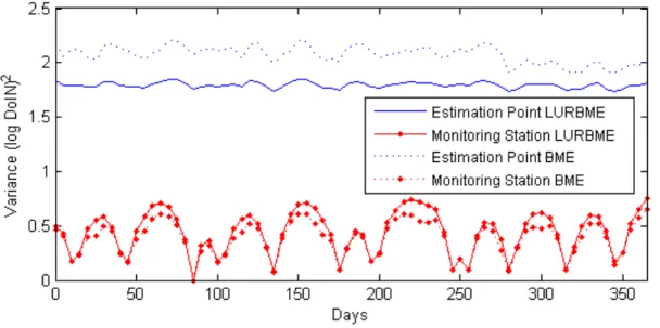
the space-time separable model. ... 17 Figure 3. Time-series of estimation error variance for 2006 at a
monitoring station (red lines) and at an estimation point where no nitrate
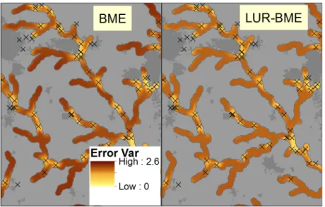
observations have been made (blue lines). ... 19 Figure 4. Error variance for log nitrate estimates In the Upper Cape Fear
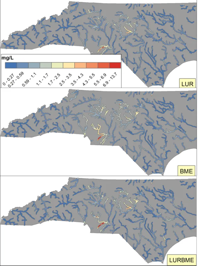
River Basin using BME (left) and LUR+BME (right) ... 20 Figure 5. Time averaged nitrate concentrations estimated by three
different models. BME figures show the time average of estimates
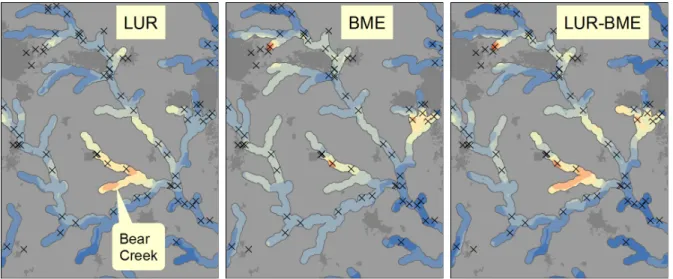
generated every five days. ... 21 Figure 6. Time averaged nitrate concentration for the Haw River
estimated by three different models. BME figures show the time
average of estimates every five days. ... 22 Figure 7. Percent reduction in nitrate concentration estimated by setting
all the percent developed open to zero. ... 33 Figure 8. Percent reduction in nitrate concentration estimated by setting
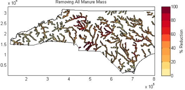
all the manure mass to zero. ... 33 Figure 9. Percent reduction in nitrate concentration estimated by setting
all the load from NPDES point sources to zero. ... 34 Figure 10. Percent reduction in nitrate concentration estimated by
setting all the waste treatment residual fields to zero. ... 34 Figure 11. Percent reduction in nitrate concentration estimated by
CHAPTER 1: INTRODUCTION
Nitrogen is an essential nutrient that is naturally occurring in various chemical forms in lakes, rivers and streams. However, through burning fossil fuels, increasing
population density, and modern farming techniques, humans have enriched nitrogen in their environment (Galloway et al. 2004). Much of this excess nitrogen eventually ends up in rivers, which transport it to downstream lakes and estuaries (Rorbert W. Howarth et al. 1996; Boyer et al. 2006; Boyer et al. 2002), where nutrient over-enrichment can lead to eutrophication (Schindler and Vallentyne 2008; Smith 1998; Paerl 1988). In estuaries and coastal areas, eutrophication due to nutrient over-enrichment is
associated with nuisance algal blooms (Paerl 1988) oxygen-depletion, or dead-zones (Rabalais et al. 2010; Diaz 2001), and harmful algal blooms (Van Dolah 2000;
Burkholder et al. 1992). In inland lakes, the role of nitrogen in eutrophication is more controversial (Schindler et al. 2008; Lewis, Wurtsbaugh, and Paerl 2011) but it does contribute to the eutrophication of several lakes in North Carolina (NCDWQ 2015; NCDWQ 2009; NCDWQ 2007).
study must be completed in order to identify the cause of impairment and create a strategy to correct the problem (USEPA 2009). These TMDL studies rely on monitoring data as well as models to guide water quality management decisions; monitoring data are also needed to track progress toward correcting water quality problems (Reckhow et al. 2001).
Because monitoring data are limited in space and time, the data are often used in conjunction with modeling to address water quality management decisions. Land use regression is commonly used to develop simple models to understand how landscape characteristics affect water quality. However, most focus on small watersheds, with perhaps a limited number of processes controlling nitrate export (Golden et al. 2009; Schoonover and Lockaby 2006; Buck, Niyogi, and Townsend 2004; Arheimer and Lidén 2000). Of the larger scale studies, most focus on nitrate (or total nitrogen) load (the product of concentration and flow) rather than concentration (Nina F Caraco and Cole 1999; Alexander et al. 2002; Hoos and McMahon 2009; McMahon, Alexander, and Qian 2003; Alexander et al. 2008). Few studies have looked at influences on nitrate
concentration from a large, very diverse set of monitoring stations (Herlihy, Stoddard, and Johnson 1998; Strayer et al. 2003; Cuevas et al. 2006; Evans et al. 2014; Schilling and Libra 2000). Land use regression studies on larger area scale are needed to understand the emergent landscape characteristics affecting water quality.
surrounding observations (Akita, Carter, and Serre 2007; Money, Carter, and Serre 2009a; Money, Carter, and Serre 2009b; Coulliette et al. 2009; Jager, Sale, and Schmoyer 1990; Li et al. 2006). Going a step further, geostatistics may be used to combine model estimates with observations, improving on estimates from either method alone (Messier et al. 2014; Messier, Akita, and Serre 2012; LoBuglio, Characklis, and Serre 2007; Yang and Jin 2010).
The objective of this study is to develop a method to estimate concentration of nitrate statewide at times and locations where it has not been observed and to use those estimates to better understand space/time variability of riverine nitrate in North Carolina. The estimate will be produced with a combination of a land use regression model and space/time geostatistics. Using the geostatistical approach provides several advantages over land use regression or watershed modeling alone. First, the estimate will be over large areas and time-dependent, providing daily estimates of nitrate
CHAPTER 2: METHODS Study Area
The study area includes rivers and streams in the state of North Carolina (Figure 1). North Carolina includes four distinct Level III EPA ecoregions (Omernik and Griffith 2014). The western, Blue Ridge region is characterized by areas of steep terrain and forest landcover. The central, Piedmont region includes large developed areas, including the Raleigh-Durham and Charlotte areas. The Piedmont also contains the headwaters of several large rivers that flow through the Plains to the Atlantic coast in North and South Carolina. The eastern, Plains regions (Southeastern and Atlantic Coastal) are characterized by flat terrain and are home to many swine feedlots.
Nitrate Data
Surface water quality in North Carolina is routinely monitored through two primary networks of stations (1) the ambient monitoring system, administered by North Carolina Department of Environment and Natural Resources, Division of Water Quality
(NCDWQ) and (2) several groups of monitoring coalitions. The goals of the ambient monitoring system are to monitor water bodies of interest, to identify locations where water quality standards are exceeded and to understand temporal and spatial water quality patterns around the state. Secondary goals support other Division of Water quality programs including basinwide water quality management plan development, biennial 305(b) and 303(d) reporting to EPA, TMDL development, and development of NPDES permit limits (Thomas 2014).
The monitoring coalitions consist of groups of stakeholders that combine resources to monitor water quality in a particular watershed. These stakeholders often include NPDES point source dischargers or drinking water permit holders that use the
monitoring to fulfill the ambient monitoring requirements associated with their permit. These data are stored in the EPA STORET databases. Samples are drawn monthly, or in some case more frequently, from water quality monitoring stations (NCDWQ 2015).
Nitrate concentrations data for all of North Carolina rivers and streams from the period 2000-2012 were downloaded from the EPA STORET website. These data are the result state ambient monitoring system, coalition monitoring, as well as field studies by EPA and its partners. The Department of water quality and coalition monitoring programs measure the total concentration nitrate (NO3-) and nitrite (NO2-) together. However, since nitrite is unstable under normal water conditions (Howarth 2010), nitrite concentrations are expected to be negligible compared to nitrate (Dubrovsky et al. 2010). For simplicity, the measured quantity “nitrate+nitrite concentrations” will be referred to as simply nitrate throughout the remainder of this document. Note that the unit of measurement is mg/L nitrate as N.
The nitrate concentrations are positively skewed with a mean of 1.16 mg/l and standard deviation 2.57 mg/l. To normalize the distribution of the data, the land use regression was completed using the natural logarithm of the time-averaged data at each station and the geostatistics were completed using the natural logarithm of the
observations. Six percent of the data were below the limit of detection, which varied from 0.001 to 0.1 mg/l, with most in the 0.01 to 0.02 mg/L range. For these data points, the value was set to half of the detection limit. The log of the temporally averaged data was used for the land use regression model, eliminating stations with fewer than 13 observations during the 13-year period, resulting 483 monitoring stations
Land Use Regression Variables
the sources of nitrate, and its transport and attenuation within the watershed (Table 1). Sources of nitrate in rivers include point sources, such as waste water treatment plants, and diffuse, non-point sources such as runoff and seepage from developed and
agricultural areas in tributary watersheds (USEPA 2009; Dubrovsky et al. 2010). The categories of variables described in Table 1, were refined and processed to create a detailed set of variables at each monitoring station. This full set of independent
variables (Appendix A) was input to a variable selection procedure, described below, to select a smaller set of independent variables used in the final land used regression model. Independent, explanatory variables for the Land Use Regression were selected from the middle of the study period (2006-2007) whenever possible to provide a general representation of conditions during the study period. For full details on processing procedures see the supplementary materials in (Messier et al. 2014).
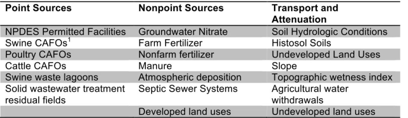
Table 1. Land Use Regression Explanatory Data
Point Sources Nonpoint Sources Transport and Attenuation
NPDES Permitted Facilities Groundwater Nitrate Soil Hydrologic Conditions
Swine CAFOs1 Farm Fertilizer Histosol Soils
Poultry CAFOs Nonfarm fertilizer Undeveloped Land Uses
Cattle CAFOs Manure Slope
Swine waste lagoons Atmospheric deposition Topographic wetness index Solid wastewater treatment
residual fields
Septic Sewer Systems Agricultural water withdrawals
Developed land uses Undeveloped land uses
variable. This hyperparameter limited the inputs to a set distance upstream from the monitoring station. The range of hyperparameters allowed was decided through
preliminary investigation that looked at the fit of linear regression using a large range of values. On plots of R2 versus range, an inflection point generally occurred around fifty kilometers, with the rate of increase in R2 very slow after 50 km. Therefore, fifty
kilometers was selected as the longest hyperparameter value in order to limit boundary effects and to limit regional effects on variable selection. The hyperparameter was used in slightly different ways for point sources and nonpoint sources.
Point sources inputs were expressed as the sum of individual sources exponentially decaying over the flow distance to the monitoring station. The predictor variable k, at estimation station i, using the kth hyperparameter is calculated as
𝑌!(!) = 𝑐0!exp −
3𝑑!"
𝜆! (1)
!"#$%&'
!!!
where 𝑐0! is the magnitude of the source m, 𝑑!" is the distance between source m and monitoring station i, and 𝜆! is the kth hyperparameter. Using this formulation sources closer to the monitoring station have a stronger influence than those farther away and sources more than 𝜆! away from the monitoring station have negligible influence.
Nonpoint sources were calculated as the sum or average of variables in the tributary watershed of a monitoring station. Hyperparameters were simply used to restrict the distance upstream from monitoring station that was considered, by using the
An additional processing step was completed for inputs represented as a mass. As a rough approximation of the dilution effect, the input mass was divided by the mean annual flow at the monitoring station. In this way, inputs to small streams should have a larger influence on concentration than inputs to large rivers.
Land Use Regression (LUR)
Time-averaged estimates of nitrate can be estimated anywhere in the state using a land use regression model. We used a nonlinear land use regression model to estimate the logarithm of the time-averaged nitrate concentrations. The nonlinear model has linear source terms modified by exponential transport and attenuation terms as given in the following equation:
𝑧! = 𝛽!+ 𝛽!𝑌!! (𝜆!)
!
!!!
exp −𝛾!𝑌!! 𝜆!
!
!!!
exp 𝛿!𝑌!! 𝜆!
!
!!!
+𝜀! (2)
where 𝑧! is the log–transform of time-averaged nitrate concentration at monitoring station i, 𝑌!! 𝜆! is the k-th source predictor variable at monitoring station i with
hyperparameter value λk, 𝛽! is the k-th source regression coefficient, 𝑌!! 𝜆! is the l-th attenuation predictor variable at monitoring station i with hyperparameter value 𝜆!, 𝛾!is the l-th attenuation regression coefficient, 𝑌!! (𝜆!) is the m-th transport predictor variable at monitoring station i with hyperparameter value 𝜆!, 𝛿! is the m-th transport regression coefficient, and εi is an error term.
model (G. E. Schwarz, Hoos, and Smith 2006). The idea behind the model is that the amount of nitrate from a give source, 𝑌!! , that reaches a monitoring will be affected by the environment through which it flows. Attenuation terms, 𝑌!! , represent soil and river conditions that promote denitrification, reducing the amount of nitrate that is observed in the stream. Transport terms, 𝑌!! , may either reduce the nitrate reaching the stream or make it easier for the nitrate to reach the stream, thereby increasing nitrate
concentrations observed.
There are important differences between the model used here and the typical SPARROW nitrogen model (e.g. Hoos and McMahon 2009; McMahon, Alexander, and Qian 2003). Firstly, instead of estimating concentration, these models estimate the load of nitrogen in rivers. Secondly, the dependent variable (load) is not log transformed. Finally, the SPARROW model is much more physically based in that nitrogen load is accumulated at points along the stream and then attenuated during transported to the next point downstream with attenuation terms representing losses that occur during that transport through streams and reservoirs that are directly included in the model. This means that (1) the dependent variable (load) in SPARROW models is more uncertain than the dependent variable used here (concentration) and (2) the SPARROW model has a much stronger physical basis than the model used here.
Model selection and fitting also followed the procedure developed by Messier et al. 2014, using the constrained forward nonlinear regression with hyperparameter
of their associated hyperparameters (𝜆’s in equation 2) to include in the land use regression model. The essential steps of the algorithm are as follows:
(1) The initial source variable is selected using a linear regression on each variable and each hyperparameter separately. The variable and its
hyperpameter that produced the best fit (based on R2) were selected as the initial source variable
(2) The initial attenuation or transport variable is selected with a nonlinear regression on each variable and its hyperparameter separately using the initial source variable selected in (1). The variable and its hyperpameter that produced fit (based on R2) were selected as the initial source variable.
(3) New variables were added in a stepwise regression. Each variable was added one at a time to the nonlinear model, the variable and its
hyperparameter that produced the best fit (based on R2) were added to the model.
(4) No more variables were added when the Bayesian Information Criterion (BIC) (Burnham 2004; G. Schwarz 1978; Aho, Derryberry, and Peterson 2014) stopped decreasing with the addition of more variables.
The model fit was evaluated with a10-fold cross-validation.
Space/time geostatistics
estimates were made using the Bayesian Maximum Entropy (BME) method of modern spatiotemporal geostastics. BME provides a method to combine general knowledge about a space/ time random field with site-specific knowledge. BME reduces to the kriging methods of linear geostatistics when the general knowledge base is restricted to the mean and covariance functions, and the data is restricted to hard data and soft data with Gaussian distributions. (G. Christakos, Bogaert, and Serre 2002; Serre and
Christakos 1999; George Christakos 1990).
To estimate point level values, we use the following procedure. Let 𝑍 𝒑 represent the space/time random field of the log nitrate across North Carolina, where 𝒑=(𝒔,𝑡) is the space (s) and time (t) coordinate.
(1) Generate a set of realizations 𝑥! of a stationary space/time random field
𝑋 𝒑 by subtracting an offset 𝑀! 𝑝! from the observed field 𝑥!
𝑥! = 𝑧! −𝑀! 𝑝! (3)
(2) Fit a covariance model to observed covariance using the generalized least squares method (Cressie 1992)
(3) Estimate 𝑥! at a new space/time location based on the general knowledge given by the covariance model from step (2) and the site-specific knowledge given by the set of observations 𝑥!
(4) Convert the estimate 𝑥! back to the variable of interest 𝑧! by adding the offset
To investigate the effect of using land use regression in the BME estimates, two choices were considered for the offset, 𝑀!(𝒑) (1) constant offset estimated by the arithmetic average of the set of observations 𝑥! (BME model) and (2) land use
CHAPTER 3: RESULTS Land Use Regression
The independent variables selected by the stepwise regression for inclusion in the time-averaged land use regression model (LUR) are summarized in Table 2. The sources variables selected include Percent Developed Open, Manure Mass, NPDES Point Source Loads, Waste Treatment Residual Fields, and Septic Sewer Density. This indicates that higher nitrate concentrations are found downstream from developed areas, areas with high agricultural animal production, and areas with high concentration of septic system usage. Higher concentrations are also found downstream from
NPDES point sources (including waste water treatment plants and industrial sources of nitrate), as well as fields where wastewater solid residuals have been applied. Percent Developed Open shows the strongest relationship with nitrate concentrations based on the single-variable R2. These results indicate that higher nitrate concentrations are associated with runoff from developed areas as well as human and animal waste.
The hyperparameter selected for source variables was always 50 km, or the longest range allowed. These source variables likely do represent regional effects, especially in the Piedmont Region, where the population of North Carolina is concentrated. In
contrast to source variables, the transport and attenuation hyperparameters are much shorter, representing effects within 2 km of the monitoring station.
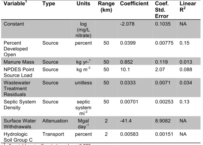
Table 2. Time-averaged Land Use Regression (LUR) variables selected for model of the log of time-averaged nitrate. For each variable, the table gives its unit, its
hyperpameter range value (km), and the value of its regression coefficient, as well as the standard error of that regression coefficient. The final column gives the R2 for single variable linear model (not the full model). Note that source variables are linear in log nitrate, while the attenuation and transport variables are exponential (equation 2).
Variable1 Type Units Range
(km)
Coefficient Coef. Std. Error
Linear R2
Constant log
(mg/L nitrate)
-2.078 0.1035 NA
Percent Developed Open
Source percent 50 0.0399 0.00775 0.15
Manure Mass Source kg yr-1 50 0.852 0.119 0.013 NPDES Point
Source Load
Source kg m-3 50 10.1 2.07 0.088
Wastewater Treatment Residuals
Source unitless 50 0.0333 0.0071 0.034
Septic System Density
Source septic system
mi-2
50 0.00701 0.00253 0.13
Surface Water Withdrawals
Attenuation Mgal
day-1 2 -41.4 8.9082 NA
Hydrologic Soil Group C
Transport percent 2 0.00583 0.00151 NA
Finally, the robustness of the variable selection procedure was confirmed with a 10-fold cross-validation (Table 4 of Appendix B), reselecting explanatory variables after removing 10% of the monitoring stations at a time. All but one of the variables selected for the overall model (Table 2) were selected ten out of ten times. The only exception the septic system density variable, which is selected seven out of ten times. This cross-validation provided strong evidence that the model is robust and supports consistent interpretation of explanatory variables across the state of North Carolina.
Space/time Geostatistics
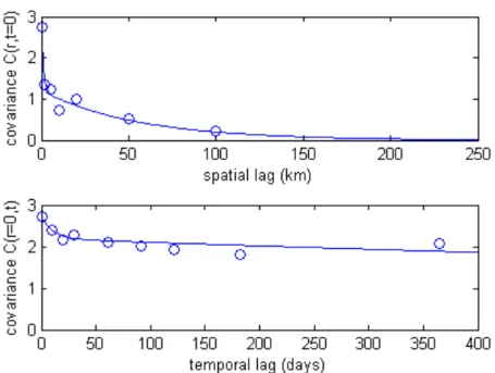
Initially, two separate covariance models were fit, consisting of a time-independent spatial model that was fit to experimental covariance values calculated based on pairs of observations that were taken on the same day, and a space-independent temporal model that was fit to experimental covariance values calculated based on pairs of observations taken at the same location (Figure 2). These two models were then combined multiplicatively to make a space/time separable model. The covariance model obtained from residuals calculated using a constant offset is given by equation (4) and the covariance model obtained from residuals calculated using the LUR offset is given in by equation (5).
model such as land use regression (LURBME), as is demonstrated by the cross-validation statistics.
Figure 2. Spatial (top) and temporal (bottom) covariance models with constant offset. The two independent models were combined to make the space-time separable model.
𝐶! 𝑟,𝜏 = 2.73 0.56 exp −
3𝑟
3.69 𝑘𝑚 +0.44exp −
3𝑟 167𝑘𝑚
∗ 0.20 exp − 3𝜏
32.0 𝑑𝑎𝑦𝑠 +0.80exp −
3𝜏
7305𝑑𝑎𝑦𝑠 (4)
𝐶! 𝑟,𝜏 =2.06 0.73exp − 3𝑟
0.252 𝑘𝑚 +0.27exp − 3𝑟
202 𝑘𝑚
∗ 0.34 exp − 3𝜏
40.9 𝑑𝑎𝑦𝑠 +0.66 exp −
3𝜏
7305𝑑𝑎𝑦𝑠 (5)
Model Comparison
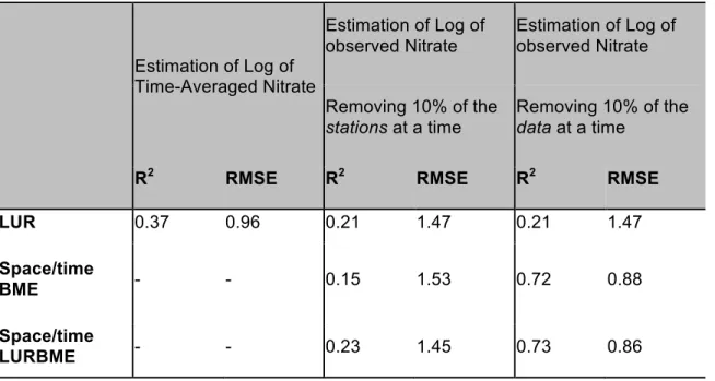
stations with no observations (center column) the LUR model and the LURBME model are almost indistinguishable, and the BME only model is not as good. However, the BME model and LURBME model do a much better job at estimating individual log nitrate observations from stations with some observations at other points in time (right column) with R2 greater that 0.7.
Table 3. 10-fold cross-validation statistics on log nitrate with (1) time-averaged data (column 1), (2) spatial cross validation (center column) and (3) temporal cross validation (right column).
Estimation of Log of Time-Averaged Nitrate
Estimation of Log of observed Nitrate
Estimation of Log of observed Nitrate
Removing 10% of the
stations at a time
Removing 10% of the
data at a time
R2 RMSE R2 RMSE R2 RMSE
LUR 0.37 0.96 0.21 1.47 0.21 1.47
Space/time
BME - - 0.15 1.53 0.72 0.88
Space/time
LURBME - - 0.23 1.45 0.73 0.86
The error variance time-series shown in Figure 3 are typical for estimates at a monitoring station and at an estimation point where no observations have been
LURBME estimate midway between sampling days because the spatial correlation is weaker for the LURBME estimate (equation 5) than for BME only (equation 4), so it derives less information from measurements taken at nearby stations.
The error variance at the estimation point (blue lines) is much higher than the error variance at the monitoring station, approaching the variance of the data itself (2.7). The error variance for the LURBME estimate is lower than the error variance for the BME only estimate because using the LUR offset reduces the variance in the residuals. The same periodicity associated with monthly sampling is also apparent in the BME
estimate, likely due to a sampling station nearby. Toward the end of the year, a sample was taken at a station near the estimation point, so we see a dip in the error variance. The LURBME estimate exhibits dampened periodicity because of the weaker spatial correlation and therefore weaker dependence on monthly measurements made nearby.
Maps of error variance averaged over the entire study period for the Haw River in central North Carolina are shown in Figure 4. The error variance away from monitoring stations is higher for the BME estimate than for the LURBME estimate, as indicated by the darker color. For both estimates, the error is smallest near the monitoring stations.
Figure 4. Error variance for log nitrate estimates In the Upper Cape Fear River Basin using BME (left) and LUR+BME (right)
CHAPTER 4: DISCUSSION
In this study, we estimate nitrate concentrations across the state of North Carolina to improve monitoring and management of nitrogen over-enrichment. The estimates are generated with space/time geostatistical method, which combines a spatial offset generated with land use regression and space/time point observations at a set of monitoring stations. The land use regression model, which estimates time-averaged nitrate concentrations across the state, identified explanatory variables related primarily to developed land use and delivery of human and animal waste. The geostatistical analysis revealed that the observations exhibit stronger temporal correlation than spatial correlation. The first contribution of this work is elucidating how the land use regression and space/time geostatistics provide complimentary methods to improve space/time point estimates of a surface water quality variable, with the land use regression improving estimates at locations where no observations are available and the
geostatistics primarily improving estimates at monitoring stations between observation times. While, the combination of a spatial model with geostatistics is not new (Messier et al. 2014; Messier, Akita, and Serre 2012; LoBuglio, Characklis, and Serre 2007; Yang and Jin 2010), this study demonstrates how the two are complimentary, with an
Land Use Regression
The second contribution of this work arises from the land use regression variable selection procedure that provides insight into the factors affecting riverine nitrogen export at a statewide scale in North Carolina. Few previous studies have been
identified that attempt to relate landscape factors to riverine nitrate concentration over such a large area using a large and diverse set of monitoring stations and no such studies have been identified for North Carolina. The scope of the study allows
interpretation of these landscape factors that are consistently related to riverine nitrate over the large area covered by North Carolina, and it provides useful insights into the emergent factors affecting riverine nitrate concentrations over this large area.
Our land use regression model identified developed land use and human and animal waste as the source variables associated with riverine nitrate (Table 2). These nitrogen sources have been identified in previous studies of riverine nitrate loading on a global scale (Nina F Caraco and Cole 1999) as well as studies of riverine total nitrogen loading for the United States and the southeastern region of the United States (McMahon, Alexander, and Qian 2003; Hoos and McMahon 2009; Preston et al. 2011). We further divide the sources into (1) Developed Areas (2) Manure Mass (3) NPDES Point Sources (including Wastewater Treatment Plants) (4) Wastewater Treatment Residual Fields and (5) the density of Septic Sewer Systems. While the first three factors are well-know sources of riverine nitrogen in North Carolina (e.g. Hoos and McMahon 2009;
generally not explicitly included in large area scale models, but it is often recognized as an important source of nitrogen to surface water locally (Jarvie et al. 2008; NCDWQ 2013; NCDWQ 2009). However, the association of land application of waste treatment residual fields with elevated concentrations of nitrate, at a statewide scale, is a new finding and a significant contribution of this work. Previous studied have associated land application of wastewater treatment residuals (also called sewage sludge or
biosolids) with elevated high nitrate concentrations in shallow groundwater (Tindall, Lull, and Gaggiani 1994) and seepage from mine reclamation sites where large volumes of biosolids have been applied or in semi-arid environments (Tian et al. 2006; Lu, He, and Stoffella 2012; Stehouwer, Day, and Macneal 2006). In North Carolina, the land
application of wastewater treatment residuals has been associated with increased groundwater nitrate concentrations at a single application site (Showers et al. 2006) and statewide (Messier et al. 2014), but this is the first study to show a large-scale
association between surface water nitrate concentration and wastewater treatment residuals.
the introduction, the dataset used for this study is expected to have a bias toward monitoring point sources (most often associated with urban areas). Second, in North Carolina, most the cultivated crops, and fertilizer application, occur in the eastern, plains regions where large rivers carry water from the headwaters in the Piedmont region to the coast. So, even if loading from farm fertilizer applications near these large rivers was significant, the effect on concentration may be minimal, due to dilution in large rivers. Third, nitrate removal processes in the landscape and in streams and wetlands may efficiently remove nitrate before it may reach the rivers; a recent SPARROW model for the southeastern US estimated that less than 12% of the nitrogen applied to
agricultural land in North Carolina is delivered to streams (Hoos and McMahon 2009). Nitrogen fertilizers may be efficiently removed by uptake from the crops that they were meant to fertilize or by denitrification processes in the landscape and in water bodies. Finally, the nitrogen from farm fertilizers may be present in rivers in other forms, such as organic nitrogen or ammonium. A preliminary analysis with total nitrogen (results not shown) suggests that this last option at least partly accounts for the missing nitrate from farm fertilizers.
Spatial and Temporal Variability of Nitrate
A movie animating maps of nitrate from 2000 to 2012 can be found at
http://www.unc.edu/depts/case/BMElab/studies/JS_N_NC/index.htm. The movie shows that some streams have consistently high concentrations but others only exhibit
transient episodes of high concentrations. Estimates of high concentration are always associated with high error (bottom frame). Two examples of streams with consistently high concentrations are shown in frames A and B at the top of the animation. Frame A shows Richardson Creek in Union County and Frame B shows Bear Creek in Chatham County. To determine the likely source of the persistent high concentrations (as
estimated by the land use regression), maps of the predicted reduction in nitrate concentration that would occur if each source variable were entirely removed from the state are given in Appendix C. For both of the highlighted streams, the likely source appears to be manure and, to a lesser extent, land application of waste treatment residuals.
Limitations and Recommendations
There are some inherent difficulties associated with modeling nitrate concentration at such a large number of monitoring stations located in diverse settings. First,
preliminary data analysis of the seasonal variability of nitrate concentrations suggested that nitrate dynamics at different stations is controlled by different processes (Appendix D). For examples, when large wastewater treatment plants are located on small
streams, as occurs for example near Greensboro and Charlotte, the average
in concentration is observed (e.g. Fayetteville). Another mechanism entirely may
influence nitrate dynamics in lakes; nitrate concentrations at monitoring stations located on lakes or just downstream from them are likely controlled by seasonal algal dynamics, with lower concentrations in late summer due to plant uptake. These differences in nutrient controlling mechanisms may be difficult to capture with a land use regression model.
Second, issues of scale may influence the sensitivity of nitrate concentrations to changes in land use in the watershed. Small streams tend to exhibit higher spatial and temporal variance than larger rivers, due to the importance of local effects (Nina F Caraco and Cole 1999 and references there in). In small streams, the stronger dependence may make the a land use regression more effective or it may be less effective simply due to the increased variability [e.g. Caraco et al., 2003; Strayer et al., 2003]. On the other hand, in large rivers, it may be difficult to disentangle the effects of different tributary areas on nutrient concentrations and nutrient removal process [e.g. Schilling and Libra, 2000].
The use of space-time geostatics in conjunction with land use regression shows great potential to provide a statewide picture of the dynamics of nutrient concentrations across the state. These estimates may be used to inform management decisions concerning nutrient regulations. In addition, the estimates may be used to improve nutrient loading estimates. Currently, nutrient loading tends to be estimated based on continuous streamflow measurements along with periodic measurements of nutrient concentrations, using a statistical method that relates concentration to streamflow or using some level of temporal averaging of streamflow, concentration or both (e.g. Cha et al. 2010; Alameddine, Qian, and Reckhow 2011; Dolan, Yui, and Geist 1981; Johnes 2007). These estimates may be improved by using a geostatistical approach. The method used here is equivalent to ordinary kriging, which provides the Best Linear Unbiased Estimate (BLUE) based on surrounding observations (Isaaks and Srivastava 1989).
APPENDIX A – LAND USE REGRESSION CANDIDATE EXPLANATORY VARIABLES
Data Description Units Variable Type Data Source
Nitrogen fertilizer applied to farmland (Average 1982-‐1997)
kg/yr nonpoint src pubs.usgs.gov/sir/2006/5012/
Sum of farm fertilizer (as above) / monitoring station flow
kg/m^3 nonpoint src pubs.usgs.gov/sir/2006/5012/
Nitrogen fertilizer applied to non-‐ farm land(Average 1982-‐1997)
kg/yr nonpoint src pubs.usgs.gov/sir/2006/5012/
Sum of non-‐farm fertilizer (as above) / monitoring station flow
kg/m^3 nonpoint src pubs.usgs.gov/sir/2006/5012/
Nitrogen in manure from livestock production (Average 1982-‐1997)
kg/yr nonpoint src pubs.usgs.gov/sir/2006/5012/
Sum of manure (as above) / monitoring station flow
kg/m^3 nonpoint src pubs.usgs.gov/sir/2006/5012/
Atmospheric Deposition (Average 1985-‐2001)
kg/yr nonpoint src pubs.usgs.gov/sir/2006/5012/
Sum of farm fertilizer (as above) / monitoring station flow
kg/m^3 nonpoint src pubs.usgs.gov/sir/2006/5012/
SwineAOP design capacity animals point source www.nconemap.com/
PoultryAOP design capacity animals point source www.nconemap.com/
Cattle AOP design capacity animals point source www.nconemap.com/
Swine Lagoons unitless point source www.nconemap.com/
Waste Treatment Residual Fields unitless point source NCDENR
2006-‐2010 Average Population Density
people/mi
^2 nonpoint src www.census.gov/
Load from NPDES Permitted Dischargers (2007)/ monitoring station flow
kg/m^3 point source cfpub.epa.gov/dmr/everyday_c riteria.cfm
Septic System Density (1990) Sewers/m
i^2 nonpoint src www.census.gov
Septic System Loading / monitoring station flow
kg/m^3 nonpoint src www.census.gov/
NLCD Open Developed percent nonpoint src www.mrlc.gov/nlcd2006.php
NLCD Low Density Developed percent nonpoint src www.mrlc.gov/nlcd2006.php
NLCD Medium Density Developed percent nonpoint src www.mrlc.gov/nlcd2006.php
NLCD High Density Developed percent nonpoint src www.mrlc.gov/nlcd2006.php
NLCD Cultivated Crops percent nonpoint src www.mrlc.gov/nlcd2006.php
NLCD Pasture/Hay percent nonpoint src www.mrlc.gov/nlcd2006.php
Soil Available Water Capacity (Layer Average)
Soil Depth to bedrock cm Transport www.soilinfo.psu.edu Hydrologic Soil Group A percent Attenuation www.soilinfo.psu.edu
Hydrologic Soil Group B percent Attenuation www.soilinfo.psu.edu
Hydrologic Soil Group C percent Transport www.soilinfo.psu.edu
Hydrologic Soil Group D percent Transport www.soilinfo.psu.edu
Soil Permeability (Layer Average) cm/hr Transport www.soilinfo.psu.edu
Soil pH pH Transport www.soilinfo.psu.edu
Percent Histosol Soils % Attenuation www.soilinfo.psu.edu
Slope unitless Transport ned.usgs.gov
Topographic Wetness Index unitless Transport ned.usgs.gov
Surface Water Withdrawals Mgal/day Transport water.usgs.gov/watuse/
Groundwater Withdrawals Mgal/day Transport water.usgs.gov/watuse/
Total Water Withdrawals Mgal/day Transport water.usgs.gov/watuse/
NLCD Deciduous Forest percent Attenuation www.mrlc.gov/nlcd2006.php
NLCD Evergreen Forest percent Attenuation www.mrlc.gov/nlcd2006.php
NLCD Forest -‐ Combined Categories
percent Attenuation www.mrlc.gov/nlcd2006.php
NLCD Mixed Forest percent Attenuation www.mrlc.gov/nlcd2006.php
NLCD Herbaceous/Grassland percent Attenuation www.mrlc.gov/nlcd2006.php
NLCD Woody Wetland percent Attenuation www.mrlc.gov/nlcd2006.php
NLCD Herbaceous Wetland percent Attenuation www.mrlc.gov/nlcd2006.php
NLCD Wetlands -‐ Combined
Categories percent Attenuation
www.mrlc.gov/nlcd2006.php
APPENDIX B – VARIABLE SELECTION VALIDATION Table 4. Variables selection 10-fold cross-validation.
Variable Type Range
(km)
Times selected
In Overall model
Constant yes
Percent Developed Open Source 50 km 10 yes
Manure Mass Source 50 km 10 yes
NPDES Point Source Load
Source 50 km 10 yes
Wastewater Treatment Residuals
Source 50 km 10 yes
Septic System Density Source 50 km 7 yes Surface Water
Withdrawals
Attenuation 2 km 10 yes
Hydrologic Soil Group C Transport 2 km 10 yes Groundwater
Withdrawals
Transport 4 km 1 no
Percent Developed Medium
Source 50 km 2 no
APPENDIX C – LAND USE REGRESSION PREDICTED REDUCTION IN TIME-AVERAGED NITRATE CONCENTRATION WITH EACH SOURCE VARIABLE
REMOVED
Figure 7. Percent reduction in nitrate concentration estimated by setting all the percent developed open to zero.
Figure 9. Percent reduction in nitrate concentration estimated by setting all the load from NPDES point sources to zero.
APPENDIX D – TIME-SERIES OF NITRATE AT SEVERAL MONITORING STATIONS
Figure 12. Station upstream from Durham WWTP on New Hope Cr.
1 2 3 4 5 6 7 8 9
x 105 0
1 2 3 4x 10
5
B3020000
Map of the monitoring stations measuring Nitrate
20000 2001 2002 2003 2004 2005 2006 2007 2008 2009 2010 2011 2012 2013 2014 0.1 0.2 0.3 0.4 0.5 Time (year) Ni tr a te ( m g /L )
Time Series of Nitrate at station B3020000
0 0.5 1 1.5 2 2.5 3 3.5 4 4.5 5
0 50 100 150 Nitrate (mg/l) Fr e q u e n c y
Figure 13. Station downstream from Durham WWTP on New Hope Cr.
1 2 3 4 5 6 7 8 9
x 105 0
1 2 3 4x 10
5
B3020000
Map of the monitoring stations measuring Nitrate
B3020000B3040000
2000 2001 2002 2003 2004 2005 2006 2007 2008 2009 2010 2011 2012 2013 2014 2 4 6 8 10 Time (year) Ni tr a te ( m g /L )
Time Series of Nitrate at station B3040000
0 2 4 6 8 10 12
0 10 20 30 40 Nitrate (mg/l) Fr e q u e n c y
Figure 14. Station on Cape Fear River downstream from Fayetteville/Ft. Bragg
1 2 3 4 5 6 7 8 9
x 105 0
1 2 3
4x 10
5
B7480000
Map of the monitoring stations measuring Nitrate
B7480000B7500000B7500000 B8290000 B7480000 B7480000B7500000B7500000 B8290000 B6370000 B6370000 B7480000 B7480000B7500000B7500000 B8290000
2000 2001 2002 2003 2004 2005 2006 2007 2008 2009 2010 2011 2012 2013 2014 0.5 1 1.5 Time (year) Ni tr a te ( m g /L )
Time Series of Nitrate at station B8290000
0 0.2 0.4 0.6 0.8 1 1.2 1.4 1.6 1.8
0 20 40 60 Nitrate (mg/l) Fr e q u e n c y
Figure 15. Station on Yadkin River at High Rock, just downstream from reservoir.
1 2 3 4 5 6 7 8 9
x 105 0
1 2 3 4x 10
5
Q7330000
Map of the monitoring stations measuring Nitrate
Q7330000Q8210000Q8210000 Q2810000 Q2810000Q2720000Q2720000Q5970000Q5970000
Q6120000
2000 2001 2002 2003 2004 2005 2006 2007 2008 2009 2010 2011 2012 2013 2014 0.2 0.4 0.6 0.8 Time (year) Ni tr a te ( m g /L )
Time Series of Nitrate at station Q6120000
0 0.1 0.2 0.3 0.4 0.5 0.6 0.7 0.8 0.9
0 5 10 15 20 25 Nitrate (mg/l) Fr e q u e n c y
REFERENCES
Aho, Ken, Dewayne Derryberry, and Teri Peterson. 2014. “Model Selection for Ecologists: The Worldviews of AIC and BIC.” Ecology 95 (3): 631–636. doi:10.1890/13-1452.1.
Akita, Yasuyuki, Gail Carter, and Marc L Serre. 2007. “Spatiotemporal Nonattainment Assessment of Surface Water Tetrachloroethylene in New Jersey.” Journal of Environmental Quality 36 (2): 508–20. doi:10.2134/jeq2005.0426.
http://www.ncbi.nlm.nih.gov/pubmed/17332255.
Alameddine, Ibrahim, Song S. Qian, and Kenneth H. Reckhow. 2011. “A Bayesian Changepoint–threshold Model to Examine the Effect of TMDL Implementation on the Flow–nitrogen Concentration Relationship in the Neuse River Basin.” Water Research 45 (1) (January): 51–62. doi:10.1016/j.watres.2010.08.003.
http://linkinghub.elsevier.com/retrieve/pii/S0043135410005671.
Alexander, Richard B, Penny J Johnes, Elizabeth W Boyer, Richard A Smith, and W Elizabeth. 2002. “A Comparison of Models for Estimationg Riverine Export of Nitrogen from Large Watersheds.” Biogeochemistry 57/58: 295–339.
Alexander, Richard B, Richard a Smith, Gregory E Schwarz, Elizabeth W Boyer, Jacqueline V Nolan, and John W Brakebill. 2008. “Differences in Phosphorus and Nitrogen Delivery to the Gulf of Mexico from the Mississippi River Basin.”
Environmental Science & Technology 42 (3) (February 1): 822–30. http://www.ncbi.nlm.nih.gov/pubmed/18323108.
Arheimer, B., and R. Lidén. 2000. “Nitrogen and Phosphorus Concentrations from Agricultural Catchments—influence of Spatial and Temporal Variables.” Journal of Hydrology 227 (1-4): 140–159. doi:10.1016/S0022-1694(99)00177-8.
Boyer, Elizabeth W, Chr Goodale, Bistine L, Norbert A Jaworski, W Robert, A Norbert, and Robert W Howarth. 2002. “Anthropogenic Nitrogen Sources and Relationships to Riverine Nitrogen Export in the Northeastern U.S.A.” Biogeochemistry 57/58: 137–169.
Boyer, Elizabeth W., Robert W. Howarth, James N. Galloway, Frank J. Dentener,
Pamela a. Green, and Charles J. Vörösmarty. 2006. “Riverine Nitrogen Export from the Continents to the Coasts.” Global Biogeochemical Cycles 20 (1): 1–9.
doi:10.1029/2005GB002537.
http://www.agu.org/pubs/crossref/2006/2005GB002537.shtml.
Buck, Oliver, Dev K. Niyogi, and Colin R. Townsend. 2004. “Scale-Dependence of Land Use Effects on Water Quality of Streams in Agricultural Catchments.”
Environmental Pollution 130 (2): 287–299. doi:10.1016/j.envpol.2003.10.018.
Burkholder, J M, E J Noga, C H Hobbs, H B Glasgow, and S A Smith. 1992. “New ‘Phantom’ Dinoflagellate Is the Causative Agent of Major Estuarine Fish Kills.” Nature. doi:10.1038/358407a0.
Burnham, K. P. 2004. “Multimodel Inference: Understanding AIC and BIC in Model Selection.” Sociological Methods & Research 33 (2): 261–304.
doi:10.1177/0049124104268644.
Caraco, N. F., J. J. Cole, G. E. Likens, G. M. Lovett, and K. C. Weathers. 2003.
“Variation in NO3 Export from Flowing Waters of Vastly Different Sizes: Does One Model Fit All?” Ecosystems 6 (4): 344–352. doi:10.1007/s10021-002-0120-x. Caraco, Nina F, and Jonathan J Cole. 1999. “Human Impact on Nitrate Export : An
Analysis Using Major World Rivers.” Ambio 28 (2): 167–170.
Cha, YoonKyung, Craig a Stow, Kenneth H Reckhow, Carlo DeMarchi, and Thomas H Johengen. 2010. “Phosphorus Load Estimation in the Saginaw River, MI Using a Bayesian Hierarchical/multilevel Model.” Water Research 44 (10) (May): 3270–82. doi:10.1016/j.watres.2010.03.008. http://www.ncbi.nlm.nih.gov/pubmed/20382406. Christakos, G., P. Bogaert, and Marc L Serre. 2002. Temporal GIS: Advanced Function
for Field-Based Applications. New York, NY: Springer.
Christakos, George. 1990. “A Bayesian/maximum-Entropy View to the Spatial Estimation Problem.” Mathematical Geology 22 (7): 763–777.
doi:10.1007/BF00890661.
Costanza, Jennifer K., Sarah E. Marcinko, Ann E. Goewert, and Charles E. Mitchell. 2008. “Potential Geographic Distribution of Atmospheric Nitrogen Deposition from Intensive Livestock Production in North Carolina, USA.” Science of the Total Environment 398 (1-3): 76–86. doi:10.1016/j.scitotenv.2008.02.024.
Coulliette, Angela D., Eric S. Money, Marc L. Serre, and Rachel T. Noble. 2009. “Space/time Analysis of Fecal Pollution and Rainfall in an Eastern North Carolina Estuary.” Environmental Science and Technology 43 (10): 3728–3735.
doi:10.1021/es803183f.
Watersheds: Trade-off between Geographic Scale, Sample Size, and Explicative Power.” Biogeochemistry 81 (3): 313–329. doi:10.1007/s10533-006-9043-5. Diaz, R J. 2001. “Overview of Hypoxia around the World.” Journal of Environmental
Quality 30 (2): 275–81. http://www.ncbi.nlm.nih.gov/pubmed/11285887.
Dolan, David M., Alexander K. Yui, and Raymond D. Geist. 1981. “Evaluation of River Load Estimation Methods for Total Phosphorus.” Journal of Great Lakes Research 7 (3): 207–214. doi:10.1016/S0380-1330(81)72047-1.
http://dx.doi.org/10.1016/S0380-1330(81)72047-1.
Dubrovsky, Neil M., Karen R. Burow, Gregory M Clark, Jann M Gronberg, Pixie A Hamilton, Kerie J. Hitt, David K. Mueller, et al. 2010. “Nutrients in the Nations Streams and Groundwater, 1992-2004.” Reston, Virginia, USA.
Evans, Daniel M., Stephen H. Schoenholtz, Parker J. Wigington, Stephen M. Griffith, and William C. Floyd. 2014. “Spatial and Temporal Patterns of Dissolved Nitrogen and Phosphorus in Surface Waters of a Multi-Land Use Basin.” Environmental Monitoring and Assessment 186: 873–887. doi:10.1007/s10661-013-3428-4.
Fry, J., G. Xian, S. Jin, J. Dewitz, C. Homer, L. Yang, C. Barnes, N. Herold, and J. Wickham. 2011. “Completion of the 2006 National Land Cover Databse for the Coterminous United States.” PE&RS 77 (9): 858–864.
Galloway, James N., Frank J. Dentener, D. G. Capone, Elizabeth W. Boyer, Robert W. Howarth, G P Asner, C C Cleveland, et al. 2004. “Nitrogen Cycles: Past, Present, and Future.” Biogeochemistry 70 (2): 153–226.
Golden, Heather E., Elizabeth W. Boyer, Michael G. Brown, S. Thomas Purucker, and René H. Germain. 2009. “Spatial Variability of Nitrate Concentrations Under Diverse Conditions in Tributaries to a Lake Watershed.” JAWRA Journal of the American Water Resources Association 45 (4) (August): 945–962.
doi:10.1111/j.1752-1688.2009.00338.x. http://doi.wiley.com/10.1111/j.1752-1688.2009.00338.x.
Herlihy, Alan T., John L. Stoddard, and Colleen Burch Johnson. 1998. “The
Relationship between Stream Chemistry and Watershed Land Cover Data in the Mid-Atlantic Region, U.S.” Water, Air, and Soil Pollution.
doi:10.1023/A:1005028803682.
Howarth, Robert W. 2010. “Inorganic Chemicals: Nitrogen.” In Biogeochemistry of Inland Waters, edited by Gene E. Likens, 400–407. Amsterdam: Elsevier.
Howarth, Rorbert W., Gilles Billen, Dennis P. Swaney, N. Townsend, K. Jawarski, Kate Lajtha, R Elmgren, et al. 1996. “Regional Nitrogen Budgets and Riverine N & P Fluxes for the Drainages to the North Atlantic Ocean: Natural and Human Influences.” Biogeochemistry 35 (1): 75–139.
http://www.springerlink.com/index/G913U054312M5G11.pdf.
Hughes, D A, and V Smakhtin. 1997. “Daily Flow Time Series Patching or Extension : A Spatial Interpolation Approach Based on Flow Duration Curves” 41 (June): 851– 872.
Isaaks, Edward H., and R. Mohan Srivastava. 1989. An Introduction to Applied Geostatistics. New York, NY: Oxford Universiyt Press.
Jager, H. I., M. J. Sale, and R. L. Schmoyer. 1990. “Cokriging to Assess Regional Stream Quality in the Southern Blue Ridge Province.” Water Resources Research 26 (7): 1401–1412. doi:10.1029/90WR00075.
Jarvie, Helen P., P. J a Withers, Robin Hodgkinson, Adam Bates, Margaret Neal, Heather D. Wickham, Sarah a. Harman, and Linda Armstrong. 2008. “Influence of Rural Land Use on Streamwater Nutrients and Their Ecological Significance.” Journal of Hydrology 350 (3-4): 166–186. doi:10.1016/j.jhydrol.2007.10.042.
Johnes, P. J. 2007. “Uncertainties in Annual Riverine Phosphorus Load Estimation: Impact of Load Estimation Methodology, Sampling Frequency, Baseflow Index and Catchment Population Density.” Journal of Hydrology 332 (1-2): 241–258.
doi:10.1016/j.jhydrol.2006.07.006.
Jordan, Thomas E, David L Correll, and Donald E Weller. 1997. “Relating Nutrient Discharges from Watersheds to Land Use and Streamflow Variability.” Water Resources Research 33 (11): 2579–2590.
Lebo, Martin E., Hans W. Paerl, and Benjamin L. Peierls. 2012. “Evaluation of Progress in Achieving TMDL Mandated Nitrogen Reductions in the Neuse River Basin, North Carolina.” Environmental Management 49 (1): 253–266. doi:10.1007/s00267-011-9774-5.
Li, Zhongwei, You Kuan Zhang, Keith Schilling, and Mary Skopec. 2006. “Cokriging Estimation of Daily Suspended Sediment Loads.” Journal of Hydrology 327 (3-4): 389–398. doi:10.1016/j.jhydrol.2005.11.028.
LoBuglio, Joseph N., Gregory W. Characklis, and Marc L. Serre. 2007. “Cost-Effective Water Quality Assessment through the Integration of Monitoring Data and Modeling Results.” Water Resources Research 43 (3): 1–16. doi:10.1029/2006WR005020. Lu, Qin, Zhenli L. He, and Peter J. Stoffella. 2012. “Land Application of Biosolids in the
USA: A Review.” Applied and Environmental Soil Science 2012. doi:10.1155/2012/201462.
McMahon, Gerard, Richard B Alexander, and Song Qian. 2003. “Support of Total Maximum Daily Load Programs Using Spatially Referenced Regression Models” (August): 315–330.
Messier, Kyle P, Yasuyuki Akita, and Marc L Serre. 2012. “Integrating Address
Geocoding, Land Use Regression, and Spatiotemporal Geostatistical Estimation for Groundwater Tetrachloroethylene.” Environmental Science & Technology 46 (5) (March 6): 2772–80. doi:10.1021/es203152a.
http://www.pubmedcentral.nih.gov/articlerender.fcgi?artid=3494280&tool=pmcentre z&rendertype=abstract.
Messier, Kyle P, Evan Kane, Rick Bolich, and Marc L Serre. 2014. “Nitrate Variability in Groundwater of North Carolina Using Monitoring and Private Well Data Models.” Environmental Science & Technology (September 2). doi:10.1021/es502725f. http://www.ncbi.nlm.nih.gov/pubmed/25148521.
Money, Eric S., Gail P. Carter, and Marc L. Serre. 2009a. “Modern Space/time Geostatistics Using River Distances: Data Integration of Turbidity and E. Coli Measurements to Assess Fecal Contamination along the Raritan River in New Jersey.” Environmental Science and Technology 43 (10): 3736–3742.
doi:10.1021/es803236j.
———. 2009b. “Using River Distances in the Space/time Estimation of Dissolved Oxygen along Two Impaired River Networks in New Jersey.” Water Research 43 (7): 1948–1958. doi:10.1016/j.watres.2009.01.034.
http://dx.doi.org/10.1016/j.watres.2009.01.034.
NCDWQ. 2015. “Monitoring Coalition Program.” Accessed September 4. http://portal.ncdenr.org/web/wq/ess/eco/coalition.
———. 2009. “Falls Lake Nutrient Response Model - Final Report.” Raleigh, North Carolina. http://portal.ncdenr.org/web/wq/ns.
———. 2013. “Study for the Ongoing Assessment of Water Quality in Jordan Lake 2013 Results.” Raleigh, North Carolina.
———. 2015. “North Carolina Nutrient Strategies.” http://portal.ncdenr.org/web/wq/ns. Nolan, Bernard T, and Kerie J Hitt. 2006. “Vulnerability of Shallow Groundwater and
Drinking-Water Wells to Nitrate in the United States.” Environmental Science & Technology 40 (24) (December 15): 7834–40.
http://www.ncbi.nlm.nih.gov/pubmed/17256535.
Omernik, James M., and Glenn E. Griffith. 2014. “Ecoregions of the Conterminous United States: Evolution of a Hierarchical Spatial Framework.” Environmental Management 54 (6): 1249–1266. doi:10.1007/s00267-014-0364-1.
http://link.springer.com/10.1007/s00267-014-0364-1.
Paerl, Hans W. 1988. “Nuisance Phytoplankton and Inland Waters ’ Blooms in Coastal , Estuarine , and Inland Waters.” Limnology and Oceanography 33: 823–847.
Preston, Stephen D, Richard B Alexander, Gregory E Schwarz, and Charles G
Crawford. 2011. “Factors Affecting Stream Nutrient Loads: A Synthesis of Regional SPARROW Model Results for the Continental United States.” Journal of the
American Water Resources Association / AWRA 47 (5) (October): 891–915. doi:10.1111/j.1752-1688.2011.00577.x.
http://www.pubmedcentral.nih.gov/articlerender.fcgi?artid=3307615&tool=pmcentre z&rendertype=abstract.
Rabalais, N. N., R. J. Díaz, L. a. Levin, R. E. Turner, D. Gilbert, and J. Zhang. 2010. “Dynamics and Distribution of Natural and Human-Caused Hypoxia.”
Biogeosciences 7 (2) (February 12): 585–619. doi:10.5194/bg-7-585-2010. http://www.biogeosciences.net/7/585/2010/.
Reckhow, Kenneth H, Anthony Donigian, James R Karr, Jan Mandrup-poulsen, Vladimir Novotny, Richard A Smith, Chris O Yoder, Leonard Shabman, Laura Ehlers, and M. Jeanne Aqulino. 2001. Assessing the TMDL Approach to Water Quality
Management. Washington, D.C.: National Academy Press. http://www.nap.edu/catalog/10146.html.
Schilling, Keith E., and Robert D. Libra. 2000. “The Relationship of Nitrate
Concentrations in Streams to Row Crop Land Use in Iowa.” Journal of Environment Quality. doi:10.2134/jeq2000.00472425002900060016x.
Schindler, David W, R E Hecky, D L Findlay, M P Stainton, B R Parker, M J Paterson, K G Beaty, M Lyng, and S E M Kasian. 2008. “Eutrophication of Lakes Cannot Be Controlled by Reducing Nitrogen Input: Results of a 37-Year Whole-Ecosystem Experiment.” Proceedings of the National Academy of Sciences of the United States of America 105 (32) (August 12): 11254–8. doi:10.1073/pnas.0805108105. http://www.pubmedcentral.nih.gov/articlerender.fcgi?artid=2491484&tool=pmcentre z&rendertype=abstract.
Schindler, David W, and John R Vallentyne. 2008. The Algal Bowl. Edmonton, Alberta, Canada: The University of Alberta Press.
Schoonover, Jon E., and B. Graeme Lockaby. 2006. “Land Cover Impacts on Stream Nutrients and Fecal Coliform in the Lower Piedmont of West Georgia.” Journal of Hydrology 331 (3-4) (December): 371–382. doi:10.1016/j.jhydrol.2006.05.031. http://linkinghub.elsevier.com/retrieve/pii/S0022169406002927.
Schwanghart, W., and D. Scherler. 2014. “Short Communication: TopoToolbox 2 – MATLAB-Based Software for Topographic Analysis and Modeling in Earth Surface Sciences.” Earth Surface Dynamics 2: 1–7. doi:10.5194/esurf-2-1-2014.
http://www.earth-surf-dynam.net/2/1/2014/.
Schwarz, G E, A B Hoos, and R A Smith. 2006. “The SPARROW Surface Water-Quality Model-Theory, Applications and User Documentation.” U.S. Geological Survey, Techniques and Methods.
Schwarz, Gideon. 1978. “Estimating the Dimension of a Model.” The Annals of Statistics 6 (2): 461–.
Serre, M L, and G Christakos. 1999. “Modern Geostatistics : Computational BME Analysis in the Light of Uncertain Physical Knowledge - the Equus Beds Study.” Stochastic Environmental Research and Risk Assessment 13 (1): 1–26.
doi:10.1007/s004770050029.
Showers, William J, Brian Usry, Matthew Fountain, John Fountain, Timothy McDade, and Dave DeMaster. 2006. “Nitrate Flux from Ground to Surface Waters Adjacent to the Neuse River Waste Water Treatment Plant.” Raleigh, North Carolina. UNC-WRRI-351-A.
Stehouwer, Richard, Rick L Day, and Kirsten E Macneal. 2006. “Nutrient and Trace Element Leaching Following Mine Reclamation with Biosolids.” Journal of Environmental Quality 35 (4): 1118–1126. doi:10.2134/jeq2005.0134.
Stow, Craig a., Mark E. Borsuk, and Donald W. Stanley. 2001. “Long-Term Changes in Watershed Nutrient Inputs and Riverine Exports in the Neuse River, North
Carolina.” Water Research 35 (6): 1489–1499. doi:10.1016/S0043-1354(00)00402-4.
Strayer, David L., R. Edward Beighley, Lisa C. Thompson, Shane Brooks, Christer Nilsson, Gilles Pinay, and Robert J. Naiman. 2003. “Effects of Land Cover on Stream Ecosystems: Roles of Empirical Models and Scaling Issues.” Ecosystems 6 (5): 407–423. doi:10.1007/s10021-002-0170-0.
Thomas, Andrea. 2014. “AMBIENT MONITORING SYSTEM ( AMS ).” Raleigh, North Carolina. http://portal.ncdenr.org/web/wq/ess/eco/ams/qapp.
Tian, G, T C Granato, R I Pietz, C R Carlson, and Z Abedin. 2006. “Effect of Long-Term Application of Biosolids for Land Reclamation on Surface Water Chemistry.”
Journal of Environmental Quality 35 (1): 101–113.
Tindall, James a., Kenneth J. Lull, and Neville G. Gaggiani. 1994. “Effects of Land Disposal of Municipal Sewage Sludge on Fate of Nitrates in Soil, Streambed Sediment, and Water Quality.” Journal of Hydrology 163 (1-2): 147–185. doi:10.1016/0022-1694(94)90027-2.
USEPA. 2015. “National Summary of Impaired Waters and TMDL Information.” Accessed January 4.
http://iaspub.epa.gov/waters10/attains_nation_cy.control?p_report_type=T#causes _303d.
———. 2009. “An Urgent Call to Action: Report of the State-EPA Nutrient Innovations Task Group.” Washington, D.C.
Van Dolah, Frances M. 2000. “Marine Algal Toxins: Origins, Health Effects, and Their Increased Occurrence.” Environmental Health Perspectives 108 (SUPPL. 1): 133– 141. doi:10.1289/ehp.00108s1143.
Yang, Xiaoying, and Wei Jin. 2010. “GIS-Based Spatial Regression and Prediction of Water Quality in River Networks: A Case Study in Iowa.” Journal of Environmental Management 91 (10): 1943–1951. doi:10.1016/j.jenvman.2010.04.011.