Approximate Frequency Counts over Data Streams

(1)

Approximate Frequency Counts over Data Streams

Gurmeet Singh Manku

Stanford University

[email protected]

Rajeev Motwani

Stanford University

[email protected]

Abstract

We present algorithms for computing frequency counts exceeding a user-specified threshold over data streams. Our algorithms are simple and have provably small memory footprints. Although the output is approximate, the error is guaranteed not to exceed a user-specified parameter. Our algo-rithms can easily be deployed for streams of single-ton items like those found in IP network monitor-ing. We can also handle streams of variable sized sets of items exemplified by a sequence of mar-ket basmar-ket transactions at a retail store. For such streams, we describe an optimized implementation to compute frequent itemsets in a single pass.

1 Introduction

In several emerging applications, data takes the form of continuous data streams, as opposed to finite stored datasets. Examples include stock tickers, network traffic measurements, web-server logs, click streams, data feeds from sensor networks, and telecom call records. Stream processing differs from computation over traditional stored datasets in two important aspects: (a) the sheer volume of a stream over its lifetime could be huge, and (b) queries re-quire timely answers; response times should be small. As a consequence, it is not possible to store the stream in its entirety on secondary storage and scan it when a query ar-rives. This motivates the design for summary data

struc-tures with small memory footprints that can support both

one-time and continuous queries.

Supported by NSF Grant IIS-0118173 and Stanford Graduate Fellowship

Supported by NSF Grant IIS-0118173, an Okawa Foundation Re-search Grant, and grants from Microsoft and Veritas.

Permission to copy without fee all or part of this material is granted pro-vided that the copies are not made or distributed for direct commercial advantage, the VLDB copyright notice and the title of the publication and its date appear, and notice is given that copying is by permission of the Very Large Data Base Endowment. To copy otherwise, or to republish, requires a fee and/or special permission from the Endowment.

Proceedings of the 28th VLDB Conference, Hong Kong, China, 2002

An aggregate query that is widely applicable is SELECT R.EventType, COUNT(*) FROM R GROUP BY R.EventType, where relation R models a stream of events with attribute R.EventTypedenoting the type of event. In several applications, groups with very low frequencies are uninteresting; the user is interested in only those groups whose frequency exceeds a certain threshold, usually expressed as a percentage of the size of the relation seen so far. The modified query then is SELECT R.EventType, COUNT(*) FROM R GROUP BY R.EventType HAVING COUNT(*) > s |R| where s is a user-specified percentage and|R|is the length of stream seen so far.

A related aggregate query is over an input stream rela-tion whose tuples are sets of items rather than individual items. The goal is to compute all subsets of items, here-after called itemsets, which occur in at least a fraction of

the stream seen so far. This is far more challenging than counting singleton tuples.

1.1 Motivating Examples

Here are four problems drawn from databases, data min-ing, and computer networks, where frequency counts ex-ceeding a user-specified threshold are computed.

1. An iceberg query [FSGM 98] performs an aggregate

function over an attribute (or a set of attributes) of a relation and eliminates those aggregate values that are below some user-specified threshold.

2. Association rules [AS94] over a dataset consisting of sets of items, require computation of frequent itemsets, where an itemset is frequent if it occurs in at least a user-specified fraction of the dataset.

3. Iceberg datacubes [BR99, HPDW01] compute only thoseGroup By’s of aCUBEoperator whose aggre-gate frequency exceeds a user-specified threshold. 4. Traffic measurement and accounting of IP packets

re-quires identification of flows that exceed a certain frac-tion of total traffic [EV01].

Existing algorithms for iceberg queries, association rules, and iceberg cubes have been optimized for finite stored data. They compute exact results, attempting to minimize the number of passes they make over the en-tire dataset. The best algorithms take two passes. When

(2)

adapted to streams, where only one pass is allowed, and results are always expected to be available with short re-sponse times, these algorithms fail to provide any a pri-ori guarantees on the quality of their output. In this paper, we present algorithms for computing frequency counts in a single pass with a priori error guarantees. Our algorithms work for variable sized transactions. We can also compute frequent sets of items in a single pass.

1.2 Offline Streams

In a data warehousing environment, bulk updates occur at regular intervals of time, e.g., daily, weekly or monthly. It is desirable that data structures storing aggregates like frequent itemsets and iceberg cubes, be maintained incre-mentally. A complete rescan of the entire database per up-date is prohibitively costly for multi-terabyte warehouses.

We call the sequence of updates to warehouses or backup devices an offline stream to distinguish it from on-line streams like stock tickers, network measurements and sensor data. Offline streams are characterized by regular bulk arrivals. Queries over these streams are allowed to be processed offline. However, there is not enough time to scan the entire database whenever an update comes along. These considerations motivate the design of summary data structures [AGP99] that allow incremental maintenance. These summaries should be significantly smaller than the base datasets but need not necessarily fit in main memory.

Query processing over offline and online streams is sim-ilar in that summary data structures need to be incremtally maintained because it is not possible to rescan the en-tire input. The difference lies in the time scale and the size of updates.

We present the first truly incremental algorithm for maintaining frequent itemsets in a data warehouse setting. Our algorithm maintains a small summary structure and does not require repeated rescans of the entire database.

1.3 Roadmap

In Section 2, we review applications that compute fre-quent itemsets, identifying problems with existing ap-proaches. In Section 3, we formally state the problem we solve. In Section 4, we describe our algorithm for singleton items. In Section 5, we describe how the basic algorithm can be extended to handle sets of items. We also describe our implementation in detail. In Section 6, we report our experiments. Related work is presented in Section 7.

2 Frequency Counting Applications

In this section, we review existing algorithms for four different applications, identifying shortcomings that sur-face when we adapt them to stream scenarios.

2.1 Iceberg Queries

The idea behind Iceberg Queries[FSGM 98] is to

iden-tify aggregates in a GROUPBYof a SQL query that exceed

a user-specified threshold . A prototypical query on a re-lationR(c1, c2, , ck, rest)with threshold is

SELECT c1, c2, , ck, COUNT(rest)

FROM R

GROUP BY c1, c2, , ck

HAVING COUNT(rest)

The parameter is equivalent tos |R|wheresis a per-centage and|R|is the size ofR. The algorithm presented in [FSGM 98] uses repeated hashing over multiple passes.

It builds upon the work of Park et al [PCY95]. The basic idea is the following: In the first pass, a set of counters is maintained. Each incoming item is hashed onto a counter which is incremented. These counters are then compressed into a bitmap, with a denoting a large counter value. In

the second pass, exact frequencies for only those elements are maintained which hash to a value whose correspond-ing bitmap value is . Variations and improvements of this

basic idea are explored in [FSGM 98]

It is difficult to adapt this algorithm for streams because at the end of the first pass, no frequencies are available.

2.2 Iceberg Cubes

Iceberg cubes [BR99, HPDW01] take Iceberg queries a step further by proposing a variant of the CUBE operator over a relationR(c1, c2, , ck, X):

SELECT c1, c2, , ck, COUNT(*), SUM(X)

FROM R

CUBE BY c1, c2, , ck

HAVING COUNT(*)

The algorithms for iceberg cubes take at least passes,

where is the number of dimensions over which the cube

has to be computed. Our algorithms can be applied as a preprocessing step to the problem of computing Iceberg Cubes. If the clause SUM(X)is removed, our algorithm can enable computation of approximate Iceberg Cubes in a single pass. We are currently exploring the application of our algorithms to Iceberg Cubes.

2.3 Frequent Itemsets and Association Rules

A transaction is defined to be a subset of items drawn from , the universe of all items. For a collection of

trans-actions, an itemset is said to have support if

occurs as a subset in at least a fraction of all transactions.

Association rules over a set of transactions are rules of the

form , where and are subsets of such that

and has support exceeding a

user-specified threshold . The confidence of a rule is

the value "!$#&%('*),+.-

$!$#&%('/-. Usually, only those rules are pro-duced whose confidence exceeds a user-specified thresh-old.

The Apriori algorithm [AS94] was one of the first suc-cessful solutions for Association Rules. The problem actu-ally reduces to that of computing frequent itemsets. Once frequent itemsets have been identified, identifying rules

(3)

whose confidence exceeds the stipulated confidence thresh-old is straightforward.

The fastest algorithms to date employ two passes. One of the first two-pass techniques was proposed by Savasere et al [SON95] where the input is partitioned into chunks that fit in main memory. The first pass computes a set of candidate frequent itemsets. The second pass computes ex-act supports for all candidates. It is not clear how this al-gorithm can be adapted for streaming data since at the end of the first pass, there are no guarantees on the accuracy of frequency counts of candidates.

Another two pass approach is based on sam-pling [Toi96]. Briefly, the idea is to produce a sample in one pass, compute frequent itemsets along with a negative

border in main memory on the samples and verify the

valid-ity of the negative border. The negative border is defined by a parameter . There is a small probability that the negative border is invalid, which happens when the frequency count of a highly-frequent element in the sample is less than its true frequency count over the entire dataset by more than . It can be shown that if we want this probability to be less than some value

, the size of the sample should be at least

, for some constant .

Toivonen’s algorithm provides strong but probabilistic guarantees on the accuracy of its frequency counts. The scheme can indeed be adapted for data streams by using reservoir sampling [Vit85]. However, there are two prob-lems: (a) false negatives occur because the error in fre-quency counts is two-sided; and, (b) for small values of , the number of samples is enormous, e.g., if , we

need over million samples. The second problem might

be ameliorated by employing concise samples, an idea first studied by Gibbons and Matias [GM98]. Essentially, re-peated occurrences of an element can be compressed into an (element, count) pair. Adapting concise samples to han-dle variable-sized transactions would amount to designing a data structure similar to FP-Trees [HPY00], which would have to be readjusted periodically as frequencies of sin-gleton items change. This idea has not been explored by the data mining community yet. Still, the problem of false negatives in Toivonen’s approach remains. Our algorithms never produce false negatives.

CARMA [Hid99] is another two-pass algorithm that gives loose guarantees on the quality of output it produces at the end of the first pass. An upper and lower bound on the frequency of each itemset is displayed to the user con-tinuously. However, there is no guarantee that the sizes of these intervals are small. CARMA provides interval infor-mation on a best-effort basis with the goal of providing the user with coarse feedback while it is running.

Online/incremental maintenance of association rules for offline streams in data warehouses is an important practical problem. We provide the first solution that is guaranteed to require no more than one pass over the entire database.

2.4 Network Flow Identification

Measurement and monitoring of network traffic is re-quired for management of complex Internet backbones. Such measurement is essential for short-term monitoring (hot spot and denial-of-service attack detection), longer term traffic engineering (rerouting traffic and upgrading selected links), and accounting (usage based pricing). Identifying flows in network traffic is important for all these applications. A flow is defined as a sequence of transport layer (TCP/UDP) packets that share the same source+destination addresses.

Estan and Verghese [EV01] recently proposed algo-rithms for identifying flows that exceed a certain threshold, say . Their algorithms are a combination of repeated

hashing and sampling, similar to those for Iceberg Queries. Our algorithm is directly applicable to the problem of net-work flow identification. It beats the algorithm in [EV01] in terms of space requirements.

3 Problem Definition

In this section, we describe our notation, our definition of approximation, and the goals of our algorithms.

Our algorithm will accept two user-specified parame-ters: a support threshold

!

, and an error parameter

such that#"

. Let$ denote the current length

of the stream, i.e., the number of tuples seen so far. In some applications, a tuple is treated as a single item. In others, it denotes a set of items. We will use the term item(set) as a short-hand for item or itemset.

At any point of time, our algorithm can be asked to pro-duce a list of item(set)s along with their estimated frequen-cies. The answers produced by our algorithm will have the following guarantees:

1. All item(set)s whose true frequency exceeds $ are

output. There are no false negatives.

2. No item(set) whose true frequency is less than &%

$

is output.

3. Estimated frequencies are less than the true frequencies

by at most $ .

Imagine a user who is interested in identifying all items whose frequency is at least(' of the entire stream seen

so far. Then (! . The user is free to set to

what-ever she feels is a comfortable margin of error. As a rule of thumb, she could set to one-tenth or one-twentieth the value of and use our algorithm. Let us assume she

chooses )! ' (one-tenth of ). As per Property ,

all elements with frequency exceeding *(' will be

output; there will be no false negatives. As per Property

+

, no element with frequency below!,- will be output.

This leaves elements with frequencies between!,- and ! . These might or might not form part of the output.

Those that make their way to the output are false positives. Further, as per property . , all individual frequencies are

less than their true frequencies by at most! .

(4)

(a) high frequency false positives, and (b) small errors in individual frequencies. Both kinds of errors are tolerable in the applications outlined in Section 2. We say that an algo-rithm maintains an -deficient synopsis if its output satisfies the aforementioned properties.

Our goal is to devise algorithms to support -deficient synopses using as little main memory as possible.

4 Algorithms for Frequent Items

In this section, we describe algorithms for computing -deficient synopses for singleton items. Extensions to sets of items will be described in Section 5. We actually de-vised two algorithms for frequency counts. Both provide the approximation guarantees outlined in Section 3. The first algorithm, Sticky Sampling, is probabilistic. It fails to provide correct answers with a miniscule probability of failure. The second algorithm, Lossy Counting, is deter-ministic. Interestingly, we experimentally show that Lossy Counting performs better in practice, although it has a the-oretically worse worst-case bound.

4.1 Sticky Sampling Algorithm

In this section, we describe a sampling based algorithm for computing an -deficient synopsis over a data stream of singleton items. The algorithm is probabilistic and is said to fail if any of the three properties in Section 3 is not satisfied. The user specifies three parameters: support ,

error and probability of failure

.

Our data structure is a set of entries of the form

, where estimates the frequency of an element

belonging

to the stream. Initially, is empty, and the sampling rate

is set to . Sampling an element with rate means that we

select the element with probability

!

. For each incoming element , if an entry for already exists in , we

incre-ment the corresponding frequency ; otherwise, we sample

the element with rate . If this element is selected by

sam-pling, we add an entry

to ; otherwise, we ignore

and move on to the next element in the stream.

The sampling rate varies over the lifetime of a stream

as follows: Let

. The first+

elements

are sampled at rate , the next

+

elements are

sam-pled at rate

+

, the next elements are sampled at rate

, and so on. Whenever the sampling rate changes,

we also scan entries in , and update them as follows: For each entry

, we repeatedly toss an unbiased coin until the coin toss is successful, diminishing by one for every

unsuccessful outcome; if becomes during this process,

we delete the entry from . The number of unsuccessful coin tosses follows a geometric distribution. Its value can be efficiently computed [Vit85]. Effectively, we have trans-formed to exactly the state it would have been in, had we been sampling with the new rate from the very beginning.

When a user requests a list of items with threshold , we

output those entries in where

%

$ .

Theorem 4.1 Sticky Sampling computes an -deficient

synopsis with probability at least %

using at most

expected number of entries.

Proof: The first+

elements find their way into . When

the sampling rate is

+

, we have$ , for some

(

. It follows that

!

#

.

Any error in the frequency count of an element

cor-responds to a sequence of unsuccessful coin tosses during the first few occurrences of . The length of this sequence

follows a geometric distribution. The probability that this length exceeds $ is at most

%

!

, which is less than

%

#

, which in turn is less than

#.

The number of elements with frequency at least is no

more than

. Therefore, the probability that the estimate for any of them is deficient by $ , is at most

. The probability of failure should be at most

. This yields!

. Since the space requirements are + , the

space bound follows. "

We call our algorithm Sticky Sampling because sweeps over the stream like a magnet, attracting all ele-ments which already have an entry in . Note that the space complexity for Sticky Sampling is independent of$ ,

the current length of the stream. The idea of maintaining counts of samples was first presented by Gibbons and Ma-tias [GM98], who used it to compress their samples and solve the Top-k problem where the most frequent items

need to be identified. Our algorithm is different in that the sampling rate increases logarithmically proportional to

the size of the stream, and that we guarantee to produce all items whose frequency exceeds , not just the top .

4.2 Lossy Counting Algorithm

In this section, we describe a deterministic algorithm that computes frequency counts over a stream of single item transactions, satisfying the guarantees outlined in Sec-tion 3 using at most

$

space where$ denotes the

current length of the stream. The user specifies two param-eters: support and error . This algorithm performs better

than Sticky Sampling in practice although theoretically, its worst-case space complexity is worse.

Definitions: The incoming stream is conceptually

di-vided into buckets of width #%$

'& transactions each.

Buckets are labeled with bucket ids, starting from . We

denote the current bucket id by (

! ! *)

#

, whose value is

$

+

& . For an element

, we denote its true frequency in

the stream seen so far by

. Note that and# are fixed

while$ ,(

! ! *)

#

and

are running variables whose val-ues change as the stream progresses.

Our data structure , is a set of entries of the form

, where is an element in the stream,

is an

inte-ger representing its estimated frequency, and- is the

max-imum possible error in .

Algorithm: Initially,, is empty. Whenever a new

ele-ment arrives, we first lookup

, to see whether an entry for already exists or not. If the lookup succeeds, we update

(5)

the entry by incrementing its frequency by one.

Other-wise, we create a new entry of the form ( !$! *) # % . We also prune, by deleting some of its entries at bucket

boundaries, i.e., whenever$

# . The rule for

deletion is simple: an entry

is deleted if

-(

! ! *)

#

. When a user requests a list of items with thresh-old , we output those entries in where

%

$ .

For an entry

, represents the exact frequency

count of ever since this entry was inserted into

, . The

value of- assigned to a new entry is the maximum

num-ber of times could have occurred in the first

( !$! *) # %

buckets. This value is exactly(

! ! *)

#

% . Once an entry

is inserted into, , its- value remains unchanged.

Lemma 4.1 Whenever deletions occur,(

! ! )

#

$ .

Lemma 4.2 Whenever an entry

gets deleted, ( ! ! *) # .

Proof: We prove by induction. Base case: (

!$! *) # . An entry

is deleted only if , which is also

its true frequency

. Thus, ( !$! *) # . Induction step: Consider an entry

that gets deleted for some (

! ! )

#

. This entry was inserted

when bucket- was being processed. An entry for

could possibly have been deleted as late as the time when bucket- became full. By induction, the true frequency of when that deletion occurred was no more than

- . Further, is the true frequency of

ever since it was inserted. It

fol-lows that

, the true frequency of in buckets

through ( ! ! *) #

, is at most - . Combined with the deletion rule

that - (

! ! )

#

, we get

( ! ! ) # . "

Lemma 4.3 If does not appear in

, , then

$ .

Proof: If the Lemma is true for an element whenever it

gets deleted, i.e., when $

# , it is true for all

other$ also. From Lemma 4.2 and Lemma 4.1, we infer

that

$ whenever it gets deleted. "

Lemma 4.4 If

, , then

$ .

Proof: If - ,

. Otherwise, was possibly

deleted sometimes in the first - buckets. From Lemma

4.2, we infer that the exact frequency of when the last

such deletion took place, is at most - . Therefore,

- . Since- (

!$! *)

#

% $ , we conclude that

$ . "

Consider elements whose true frequency exceeds $ .

There cannot be more than

such elements. Lemma 4.3

shows that all of them have entries in, . Lemma 4.4 further

shows that the estimated frequencies of all such elements are accurate to within $ . Thus, , correctly maintains

an -deficient synopsis. The next theorem shows that the number of low frequency elements (which occur less than

$ times) is not too large.

Theorem 4.2 Lossy Counting computes an -deficient

syn-opsis using at most

$

entries.

Proof: Let (

!$! *)

#

be the current bucket id. For each

( , let denote the number of entries in, whose

bucket id is %

. The element corresponding to such an

entry must occur at least

times in buckets %

through ; otherwise, it would have been deleted. Since the size of

each bucket is# , we get the following constraints:

# +

& (1)

We claim that

# + (2)

We prove Inequality (2) by induction. The base case

follows from Inequality (1) directly. Assume

that Inequality (2) is true for

+

& % . We

will show that it is true for ! as well. Adding

In-equality (1) for " to % instances of

Inequal-ity (2) (one each for

varying from to % ) gives

us # $# %# '&(&)& *# # # + # + *&(&(& # +

. Upon rear-rangement, we get #

+ # # % -+ which

then readily simplifies to Inequality (2) for , , thereby

completing the induction step. Since -,.- /#10

, from Inequality 2, we get -,.-2 # 0 + $ "

If we make the assumption that in real world datasets, elements with very low frequency (at most

) tend to

oc-cur more or less uniformly at random, then Lossy Count-ing requires no more than 3 space, as proved in the

Ap-pendix. We note that the IBM test data generator for data mining [AS94] for generating synthetic datasets for associ-ation rules, indeed chooses low frequency items uniformly randomly from a fixed distribution.

4.3 Sticky Sampling vs Lossy Counting

In this section, we compare Sticky Sampling and Lossy Counting. We show that Lossy Counting performs signifi-cantly better for streams with random arrival distributions.

A glance at Theorems 4.1 and 4.2 suggests that Sticky Sampling should require constant space, while Lossy Counting should require space that grows logarithmically with$ , the length of the stream. However, these theorems

do not tell the whole story because they bound worst-case space complexities. For Sticky Sampling, the worst case amounts to a sequence with no duplicates, arriving in any order. For Lossy Counting, the worst case corresponds to a rather pathological sequence that we suspect would almost never occur in practice. We now show that if the arrival or-der of the elements is uniformly random, Lossy Counting is superior by a large factor.

We studied two streams. One had no duplicates. The other was highly skewed and followed the Zipfian distri-bution. Most streams in practice would be somewhere in

(6)

between in terms of their frequency distributions. For both streams, we assumed uniformly random arrival order.

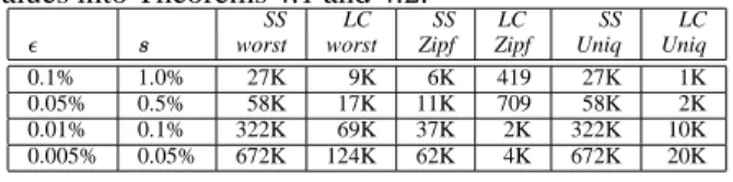
Table 1 compares the two algorithms for varying values of . The value of is consistently chosen to be one-tenth of . Worst case space complexities are obtained by plugging

values into Theorems 4.1 and 4.2.

SS LC SS LC SS LC

worst worst Zipf Zipf Uniq Uniq

0.1% 1.0% 27K 9K 6K 419 27K 1K

0.05% 0.5% 58K 17K 11K 709 58K 2K

0.01% 0.1% 322K 69K 37K 2K 322K 10K

0.005% 0.05% 672K 124K 62K 4K 672K 20K

Table 1: Memory requirements in terms of number of entries. LC de-notes Lossy Counting. SS dede-notes Sticky Sampling. Worst dede-notes worst-case bound. Zipf denotes Zipfian distribution with parameter

. Uniq denotes a stream with no duplicates. Length of stream .

Proba-bility of failure .

Figure 1 shows the amount of space required for the two streams as a function of$ , with support , error ! , and probability of failure

. The kinks in the curve for Sticky Sampling correspond to re-sampling. They are

+

units apart on the X-axis. For kinks for Lossy Counting correspond to bucket boundaries when deletions occur.

0 5000 10000 15000 20000 25000 30000

2 3 4 5 6 7

No of entries

Log10 of Stream length N Comparison of Memory Requirements

Sticky Sampling (Uniq) Sticky Sampling (Zipf) Lossy Counting (Uniq) Lossy Counting (Zipf)

0 200 400 600 800 1000 1200 1400

0 2000 4000 6000 8000 10000

No of entries

Stream length N

Memory Requirement Profile for Lossy Counting Lossy Counting (Uniq)

Lossy Counting (Zipf)

Figure 1:Memory requirements in terms of number of entries for sup-port

, error

, probability of failure

. Zipf denotes a Zipfian distribution with parameter

. Uniq denotes a stream with no duplicates. The bottom figure magnifies a section of the barely visible lines in the upper graph.

Sticky Sampling performs worse because of its ten-dency to remember every unique element that gets sam-pled. Lossy Counting, on the other hand, is good at prun-ing low frequency elements quickly; only high frequency elements survive. For highly skewed data, both algorithms require much less space than their worst-case bounds.

4.4 Comparison with Alternative Approaches

A well-known technique for estimating frequency counts employs uniform random sampling. If the sample size is at least

, the relative frequency of any single

element is accurate to within a fraction , with probability at least&%

. This basic idea was used by Toivonen [Toi96] to devise a sampling algorithm for association rules. Sticky Sampling beats this approach by roughly a factor of

.

Another algorithm for maintaining -deficient synopsis can employ -approximate quantiles [MRL99]. The key idea is that an element with frequency exceeding will

recur several times if is small relative to . It follows

that if we set !

, and compute -approximate

his-tograms, high frequency elements can be deduced to within an error of . Using the algorithm due to Greenwald and Khanna [GK01], the worst-case space requirement would be

+

$

, worse than that for Lossy Counting, as per Theorem 4.2. Also, it is not obvious how quantile algo-rithms can be efficiently extended to handle variable-sized

sets of items, a problem we consider in Section 5.

We recently learned about an as yet unpublished algo-rithm [KPS02] for identifying elements whose frequency exceeds a fraction of the stream. The algorithm com-putes exact counts in two passes. However, the essential ideas can be used to maintain an -deficient synopsis us-ing exactly

space. In the first pass, the algorithm

main-tains

elements along with their counters. Initially, all

counters are free. Whenever a new element arrives, we check if a counter for this element exists. If so, we sim-ply increment it. Otherwise, if a counter is free, it is as-signed to this element with initial value . If all counters

are in use, we repeatedly diminish all

counters by

un-til some counter becomes free, i.e., its value drops to zero. Thereafter, we assign the newly arrived element a counter with initial value . This algorithm works for streams of

singleton items. However, there does not appear to be a straightforward adaptation to the scenario where a stream of variable-sized transactions is being analyzed and the dis-tribution of transaction sizes is not known. Moreover, if the input stream is Zipfian, the number of elements exceed-ing the threshold is significantly smaller than

. Table 1

shows that Lossy Counting actually takes much less than

space. For example, with , roughly

+

entries

suffice, which is only+

- of

. The skew in the

frequen-cies is even more when we consider the problem of iden-tifying frequent sets of items in Section 5. For example, assume that all transactions are known to have a fixed size

and that frequent subsets of size. are being computed.

An adaptation of algorithm [KPS02] would maintain

#"%$ &!'

counters. Lossy Counting would require significantly less space, as experiments in Section 6 show.

5 Frequent Sets of Items

– From Theory to Practice

In this section, we develop a Lossy Counting based al-gorithm for computing frequency counts over streams that

(7)

consist of sets of items. This section is less theoretical in nature than the preceding one. The focus is on system-level issues and implementation artifices for optimizing memory and speed.

5.1 Frequent Itemsets Algorithm

The input to the algorithm is a stream of transactions where each transaction is a set of items drawn from . We

denote the current length of this stream by $ . The user

specifies two parameters: support , and error . The

chal-lenge lies in handling variable sized transactions and avoid-ing explicit enumeration of all subsets of any transaction.

Our data structure , is a set of entries of the form

, where

is a subset of items, is an

inte-ger representing its approximate frequency, and - is the

maximum possible error in . Initially,, is empty.

Imagine dividing the incoming transaction stream into

buckets, where each bucket consists of#

$

'&

transac-tions. Buckets are labeled with bucket ids, starting from

. We denote the current bucket id by (

! ! )

#

. We do not process the input stream transaction by transaction. In-stead, we try to fill available main memory with as many transactions as possible, and then process such a batch of transactions together. This is where the algorithm differs from that presented in Section 4.2. Over time, the amount of main memory available might increase/decrease. Let denote the number of buckets in main memory in the cur-rent batch being processed. We update, as follows:

UPDATESET: For each entry

, ,

up-date by counting the occurrences of in the current

batch. If the updated entry satisfies - (

!$! *)

#

, we delete this entry.

NEW SET: If a set

has frequency in the

current batch and

does not occur in, , create a new

entry

(

! ! *)

#

%

. It is easy to see that every set

whose true

fre-quency

#

$ , has an entry in, . Also, if an entry

, , then, the true frequency

#

satisfies the

inequality

#

- . When a user requests a list of

items with threshold , we output those entries in, where

%

$ .

It is important that be a large number. The reason is that any subset of that occurs times or more,

contributes an entry to, . For a smaller , more spurious

subsets find their way into, .

In the next section, we show how, can be represented

compactly and how UPDATESET and NEW SET can be implemented efficiently.

5.2 Data Structures

Our implementation has three modules: BUFFER, TRIE, and SETGEN. BUFFERrepeatedly reads in a batch of trans-actions into available main memory. TRIEmaintains the data structure , described earlier. SETGEN operates on

the current batch of transactions. It enumerates subsets of these transactions along with their frequencies. Together

with TRIE, it implements the UPDATE SETand NEW SET

operations. The challenge lies in designing a space efficient representation of TRIE and a fast algorithm for SETGEN

that avoids generating all possible subsets of itemsets.

Buffer: This module repeatedly reads in a batch of

transactions into available main memory. Transactions are sets of item-id’s. They are laid out one after the other in a big array. A bitmap is used to remember transaction bound-aries. A bit per per item-id denotes whether this item-id is the last member of some transaction or not. After reading in a batch, BUFFERsorts each transaction by its item-id’s.

Trie: This module maintains the data structure,

out-lined in Section 5.1. Conceptually, it is a forest (a set of trees) consisting of labeled nodes. Labels are of the form

, where

is an item-id, is its

estimated frequency,- is the maximum possible error in ,

and

is the distance of this node from the root of the

tree it belongs to. The root nodes have level . The level of

any other node is one more than that of its parent. The chil-dren of any node are ordered by their item-id’s. The root nodes in the forest are also ordered by item-id’s. A node in the tree represents an itemset consisting of item-id’s in that node and all its ancestors. There is a to mapping

between entries in, and nodes in TRIE.

Tries are used by several Association Rules algorithms. Hash tries [AS94] are a popular choice. Usual implemen-tations of, as a trie would require pointers and

variable-sized memory segments (because the number of children of a node changes over time).

Our TRIEis different from traditional implementations. Since tries are the bottleneck as far as space is con-cerned, we designed them to be as compact as possi-ble. We maintain TRIE as an array of entries of the form

- corresponding to the pre-order

traversal of the underlying trees. Note that this is

equiva-lent to a lexicographic ordering of the subsets it encodes. There are no pointers from any node to its children or its siblings. The

’s compactly encode the underlying tree

structure. Our representation is okay because tries are al-ways scanned sequentially, as we show later.

SetGen: This module generates subsets of item-id’s

along with their frequencies in the current batch of trans-actions in lexicographic order. Not all possible subsets need to be generated. A glance at the description of UP

-DATE SETand NEW SET operations reveals that a subset must be enumerated iff either it occurs in TRIEor its fre-quency in the current batch exceeds . SETGENuses the following pruning rule:

If a subset does not make its way into TRIE

af-ter application of both UPDATE SETand NEW SET, then no supersets of should be considered.

This is similar to the Apriori pruning rule. We describe an efficient implementation of SETGENin greater detail later.

Overall Algorithm

(8)

many transactions as possible, and sorts them. SETGEN

operates on the current batch of transactions. It generates sets of itemsets along with their frequency counts in lexi-cographic order. It limits the number of subsets using the pruning rule. Together, TRIEand SETGENimplement the UPDATE SETand NEW SEToperations. In the end, TRIE

stores the updated data structure, , and BUFFERgets ready

to read in the next batch.

5.3 Efficient Implementations

Buffer: If item-id’s are successive integers from thru

- -, and if is small enough (say, less than million), we

maintain exact frequency counts for singleton sets. If- - , we need an array of size only

. When

ex-act frequency counts are maintained, BUFFERfirst prunes away those item-id’s whose frequency is less than $ , and

then sorts the transactions. Note that$ is the length of the

stream up to and including the current batch of transactions.

Trie: As SETGENgenerates its sequence of sets and

as-sociated frequencies, TRIE needs to be updated. Adding or deleting TRIEnodes in situ is made difficult by the fact

that TRIEis a compact array. However, we take advantage of the fact that the sets produced by SETGEN(and there-fore, the sequence of additions and deletions) are lexico-graphically ordered. Recall that our compact TRIEstores its constituent subsets in their lexicographic order. This lets SETGENand TRIEwork hand in hand.

We maintain TRIEnot as one huge array, but as a set of fairly large-sized chunks of memory. Instead of modify-ing the original trie, we create a new TRIEafresh. Chunks from the old TRIE are freed as soon as they are not re-quired. Thus, the overhead of maintaining two Tries is not significant. By the time SETGENfinishes, the chunks of the original trie have been completely discarded.

For finite streams, an important TRIEoptimization per-tains to the last batch of transactions when the value of , the number of buckets in BUFFER, could be small. Instead of applying the rules in Section 5.1, we prune nodes in the trie more aggressively by setting the threshold for deletion to instead of(

! ! *)

#

. This is because the lower

frequency nodes do not contribute to the final output.

SetGen: This module is the bottleneck in terms of time

for our algorithm. Optimizing it has made it fairly complex. We describe the salient features of our implementation.

SETGENemploys a priority queue called Heap which initially contains pointers to smallest item-id’s of all trans-actions in BUFFER. Duplicate members (pointers pointing to the same item-id) are maintained together and they con-stitute a single entry in Heap. In fact, we chain all the point-ers together, deriving the space for this chain from BUFFER

itself. When an item-id in BUFFERis inserted into Heap, the -byte integer used to represent an item-id is converted

into a -byte pointer. When a heap entry is removed, the

pointers are restored back to item-id’s.

SETGEN repeatedly processes the smallest item-id in

Heap to generate singleton sets. If this singleton belongs

to TRIEafter UPDATE SETand NEW SETrules have been applied, we try to generate the next set in lexicographic se-quence by extending the current singleton set. This is done by invoking SETGENrecursively with a new heap created out of successors of the pointers to item-id’s just removed and processed. The successors of an item-id is the item-id following it in its transaction. Last item-id’s of transactions have no successors. When the recursive call returns, the smallest entry in Heap is removed and all successors of the currently smallest item-id are added to Heap by following the chain of pointers described earlier.

5.4 System Issues and Optimizations

BUFFER scans the incoming stream by memory map-ping the input file. This saves time by getting rid of double copying of file blocks. The UNIX system call for mem-ory mapping files is mmap(). The accompanying

mad-vise()interface allows a process to inform the operating

systems of its intent to read the file sequentially. We used the standardqsort()to sort transactions. The time taken to read and sort transactions pales in comparison with the time taken by SETGEN, obviating the need for a custom sort routine. Threading SETGEN and BUFFER does not help because SETGENis significantly slower.

Tries are written and read sequentially. They are oper-ational when BUFFERis being processed by SETGEN. At this time, the disk is idle. Further, the rate at which tries are scanned (read/written) is much smaller than the rate at which sequential disk I/O can be done. It is indeed possible to maintain TRIEon disk without any loss in performance. This has two important advantages:

(a) The size of a trie is not limited by the size of main memory available, as is the case with other algorithms. This means that our algorithm can function even when the amount of main memory available is quite small. (b) Since most available memory can be devoted to

BUFFER, we can work with smaller values of than other algorithms can handle. This is a big win. TRIE is currently implemented as a pair of anony-mous memory mapped segments. They can be associated with actual files, if the user so desires. Since tries are read/written sequentially, as against being accessed ran-domly, it is possible to compress/decompress it on the fly as sections of it are read/written to disk. Our current im-plementation does not attempt any compression; we use fourint’s for node labels. Writing TRIEto disk violates a pedantic definition of single-pass algorithms. However, we should note that the term single-pass is meaningful only for disk-bound applications. Our program is cpu-bound.

Memory requirements for Heap are modest. Available main memory is consumed primarily by BUFFER, assum-ing TRIEare on disk. Our implementation allows the user to specify the size of BUFFER.

(9)

5.5 Novel Features of our Technique

Our implementation differs from Apriori and its variants in one important aspect: there is no candidate generation phase. Apriori first finds all frequent itemsets of size

be-fore finding frequent itemsets of size . This amounts

to a breadth first search of the frequent itemsets on a lattice. Our algorithm carries out a depth first search. Incidentally, BUC [BR99] also uses repeated depth first traversals for Iceberg Cube computation. However, it makes passes

over the entire data where is the number of dimensions in

the cube.

The idea of using compact disk-based tries is novel. It allows us to compute frequent itemsets under low memory conditions. It also enables our algorithm to handle smaller values of support threshold than previously possible.

6 Experimental Results

We experimented with two kinds of datasets: streams of market-basket transactions, and text document sequences.

6.1 Frequent Itemsets over Streams of Transactions

Our experiments were carried out on the IBM test data generator [AS94]. We study two data-streams of size

mil-lion transactions each. One has an average transaction size of with average large itemset size of . The other has

av-erage transaction size and average large itemset size .

Following the conventions set forth in [AS94], the names of

the datasets are ! ( and ! , where

the three numbers denote the average transaction size ( ),

the average large itemset size ( ) and the number of

trans-actions respectively. Items were drawn from a universe of

unique items. The raw sizes of the two streams

were, MB and, MB respectively. All experiments were

carried out on a ,.. Pentium III processor running

Linux Kernel version 2.2.16.

In our experiments, we always fix ! (one-tenth

of ). Moreover, the amount of main memory required by

our programs is dominated by BUFFER, whose size is stipu-lated by the user. We are then left with four parameters that we study in our experiments: support , number of

transac-tions$ , size of BUFFER, and total time taken. We measure

wall clock time.

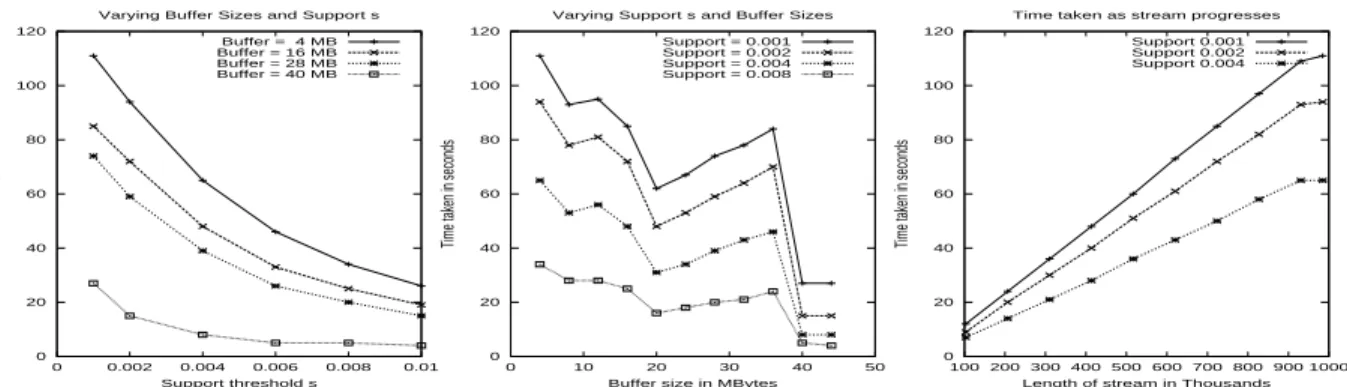
In Figure 2, we plot times taken by our algorithm for values of support ranging from(' to , and BUFFER

size ranging from MB to MB. The leftmost graphs

show how decreasing leads to increases in running time.

The kinks in the middle graphs in Figure 2 have an in-teresting explanation. The graphs plot running time for varying BUFFER sizes. For a fixed value of support ,

the running time sometimes increases as BUFFERsize in-creases. This happens due to a TRIEoptimization we de-scribed in Section 5.3. For finite streams, when the last batch of transactions is being processed, the threshold is raised to $ . This leads to considerable savings in the

run-ning time of the last batch. In Figure 2, when BUFFER

size is+

, the input is split into only two (almost equal

sized) batches. As BUFFER size increases, the first batch increases in size, leading to an increase in running time. Fi-nally, when BUFFERsize reaches MB, it is big enough to

accommodate the entire input as one batch, which is rapidly processed. This leads to a sharp decrease in running time. Increasing BUFFER size further has no effect on running time.

The rightmost graphs in Figure 2 show that the running time is linearly proportional to the length of the stream. The curve flattens in the end as processing the last batch is faster owing to the TRIEoptimization mentioned in Section 5.3.

The disk bandwidth required to read the input file was always less than MBps. This is a very low rate when

com-pared with modern day disks. A single high performance SCSI disk can deliver between +

and MBps. This

confirms that frequent itemset computation is cpu bound. An interesting fact that emerged from our experiments was that the error in the output was almost zero. Over,,

of the itemsets reported in the output had error. This

happens because a highly frequent itemset invariably oc-curs within the first batch of transactions. Once it enters our data structure, it is very unlikely to get deleted. There are rarely any false positives for the same reason (the fre-quencies of all elements in the range

%

are also accurate). This suggests that we might be able to set to a higher value and still get accurate results. A higher error rate might be observed in highly skewed data or if global data characteristics change, e.g. if the stream is sorted.

Comparison with Apriori

For comparison with the well known Apriori Algo-rithm [AS94], we down-loaded a publicly available pack-age written by Christian Borgelt

. It is a pretty fast im-plementation of Apriori using prefix trees and is used in a commercial data mining package. Since the version of Linux we used did not supportmallinfo, we re-linked Borgelt’s program with the widely available dlmalloc library by Doug Lea

. We invokedmallinfojust before program termination to figure out its memory requirements.

Our algorithm Our algorithm Apriori with 4MB Buffer with 44MB Buffer Support Time Memory Time Memory Time Memory

0.001 99 s 81.96 MB 111 s 12.49 MB 27 s 45.16 MB 0.002 25 s 53.34 MB 94 s 9.92 MB 15 s 45.02 MB 0.004 14 s 48.09 MB 65 s 7.20 MB 8 s 45.00 MB 0.006 13 s 47.87 MB 46 s 6.03 MB 6 s 44.98 MB 0.008 13 s 47.86 MB 34 s 5.53 MB 4 s 44.95 MB 0.010 14 s 47.86 MB 26 s 5.22 MB 4 s 44.93 MB Table 2: Performance comparison for ! (

which has

transactions over unique items with

average transaction size .

In Table 2, we compare Apriori with our algorithm for the dataset ! ( , varying support from(' to . Error was set at of . We ran our

algo-rithm twice, first with BUFFERset to MB, and then, with

http://fuzzy.cs.uni-magdeburg.de/˜borgelt/ software.html

(10)

0 20 40 60 80 100 120

0 0.002 0.004 0.006 0.008 0.01

Time taken in seconds

Support threshold s Varying Buffer Sizes and Support s

Buffer = 4 MB Buffer = 16 MB Buffer = 28 MB Buffer = 40 MB

0 20 40 60 80 100 120

0 10 20 30 40 50

Buffer size in MBytes Varying Support s and Buffer Sizes

Support = 0.001 Support = 0.002 Support = 0.004 Support = 0.008

0 20 40 60 80 100 120

100200 300400500600 700800900 1000

Length of stream in Thousands Time taken as stream progresses

Support 0.001 Support 0.002 Support 0.004

(a) Times taken for IBM test dataset with items. No of transactions$ was million.

0 100 200 300 400 500 600 700 800 900 1000

0 0.002 0.004 0.006 0.008 0.01

0 100 200 300 400 500 600 700 800 900 1000

0 10 20 30 40 50

Support = 0.001 Support = 0.002 Support = 0.004 Support = 0.008

0 100 200 300 400 500 600 700 800 900 1000

0 100 200 300 400 500 600 700 800 9001000

(b) Times taken for IBM test dataset ( with items. No of transactions$ was million.

Figure 2: Experimental results for our algorithm over IBM test datasets.

0 200 400 600 800 1000 1200

0.004 0.008 0.012 0.016 0.02

0 200 400 600 800 1000 1200

0 5 10 15 20

Support = 0.005 Support = 0.007 Support = 0.010 Support = 0.015 Support = 0.020

0 200 400 600 800 1000 1200

10 20 30 40 50 60 70 80 90

(a) Times taken for frequent word-pairs in 100K web pages.

0 500 1000 1500 2000

0 0.004 0.008 0.012 0.016 0.02

0 500 1000 1500 2000

0 5 10 15 20 25 30

Support = 0.004 Support = 0.008 Support = 0.012 Support = 0.016 Support = 0.020

0 200 400 600 800 1000 1200 1400 1600 1800

200 400 600 800

(b) Times taken for frequent word-pairs in 800K Reuters documents Figure 3: Times taken for Iceberg Queries over Web pages and Reuters articles.

(11)

BUFFERset to MB. The table shows the total memory required by the two programs. For our program, this in-cludes the maximum cost of HEAPand TRIE, during run-time. As the value of support increases, the memory

re-quired by TRIEdecreases. This is because there are fewer itemsets with higher support. The size of the TRIE also decreases when BUFFER changes from MB to MB.

This is because the value of (see Section 5.1) increases. Therefore, there are fewer low frequency subsets (with fre-quency less than ) that creep into the trie. It is interesting to observe that with BUFFER set to a small value, MB,

our algorithm was able to compute all frequent itemsets us-ing much less memory than Apriori but more time. With

BUFFERsize MB, the entire input fits in main memory. Our program beats Apriori be a factor of +

to. showing

that our main memory implementation is much faster.

6.2 Iceberg Queries

An iceberg query studied in [FSGM 98] was the

iden-tification of all pairs of words in a repository of !

web documents which occur at least times

to-gether. Note that the relation for this query is not explic-itly materialized. This query is equivalent to identifying all word pairs that occur in at least of all documents.

We ran this query over two different datasets.

The first dataset was a collection of web pages

crawled by WebBase, a web crawler developed at Stanford University [HRGMP00]. Words in each document were identified. Common stop-words [SB88] were removed. The resulting input file was MB. Experiments for this

dataset were carried out on a 933 MHz Pentium III ma-chine running Linux Kernel version 2.2.16.

The second dataset was the well-known Reuters news-wire dataset, containing news articles. The input

file resulting from this dataset after removing stop-words was roughly +

MB. Experiments for this dataset were

carried out on a 700 MHz Pentium III machine running Linux Kernel version 2.2.16.

We study the interplay of$ , the length of the stream, ,

the support, time taken, and the size of BUFFERin Figure 3. The overall shape of the graphs is very similar to those for frequent itemsets over the IBM test datasets that we studied in the previous section.

For the sake of comparison with the algorithm presented in the original Iceberg Queries paper [FSGM 98], we ran

our program over web documents with support ! . This settings corresponds to the first query

studied in [FSGM 98] (see Figure in their paper). We

ran our program on exactly the same machine, a 200 MHz Sun Ultra/II with 256 MB RAM running SunOS 5.6. We fixed BUFFER at MB. Our program processed the

in-put in batches, producing., frequent word pairs.

BUFFER, Heap and auxiliary data structures required +

MB. The maximum size of a trie was MB. Our program

took seconds to complete. Fang et al [FSGM 98]

re-port that the same query required over' seconds using

roughly. MB main memory. Our algorithm is faster.

An interesting duality emerges between our approach and that of the algorithm in [FSGM 98]. Our program

scans the input just once, but repeatedly scans a temporary file on disk (the memory mapped TRIE). The Iceberg algo-rithm scans the input multiple times, but uses no temporary storage. The advantage in our approach is that it does not require a lookahead into the data stream.

7 Related and Future Work

Problems related to frequency counting that have been studied in the context of data streams include approximate frequency moments [AMS96],

differences [FKSV99], distinct values estimation [FM85, WVZT90], bit count-ing [DGIM02], and top-k queries [GM98, CCFC02]. Algorithms over data streams that pertain to aggrega-tion include approximate quantiles [MRL99, GK01], V-optimal histograms [GKS01b], wavelet based aggregate queries [GKMS01, MVW00], and correlated aggregate queries [GKS01a].

We are currently exploring the application of our basic techniques to sliding windows, data cubes, and two-pass algorithms for frequent itemsets.

8 Conclusions

We proposed novel algorithms for computing approx-imate frequency counts of elements in a data stream. Our algorithms require provably small main memory footprints. The problem of identifying frequent elements is at the heart of several important problems: iceberg queries, frequent itemsets, association rules, and packet flow identification. We can now solve each of them over streaming data.

We also described a highly optimized implementation for identifying frequent itemsets. In general, our algorithm produces approximate results. However, for the datasets we studied, our algorithm runs in one pass and produces exact results, beating previous algorithms in terms of time.

Our frequent itemsets algorithm can handle smaller val-ues of support threshold than previously possible. It re-mains practical even in environments with moderate main memory. We believe that our algorithm provides a practi-cal solution to the problem of maintaining association rules incrementally in a warehouse setting.

References

[AGP99] S. ACHARYA, P. B. GIBBONS,ANDV. POOSALA. Aqua: A fast decision support system using approximate query answers. In Proc. of 25th Intl. Conf. on Very Large Data

Bases, pages 754–755, 1999.

[AMS96] N. ALON, Y. MATIAS,AND M. SZEGEDY. The space complexity of approximating the frequency moments. In

Proc. of 28th Annual ACM Symp. on Theory of Computing,

pages 20–29, May 1996.

[AS94] R. AGRAWAL ANDR. SRIKANT. Fast algorithms for min-ing association rules. In Proc. of 20th Intl. Conf. on Very

Large Data Bases, pages 487–499, 1994.

[BR99] K. BEYER ANDR. RAMAKRISHNAN. Bottom-up compu-tation of sparse and iceberg cubes. In Proc. of 1999 ACM

(12)

[CCFC02] M. CHARIKAR, K. CHEN, ANDM. FARACH-COLTON. Finding frequent items in data streams. In Proc. 29th Intl.

Colloq. on Automata, Languages and Programming, 2002.

[DGIM02] M. DATAR, A. GIONIS, P. INDYK,ANDR. MOTWANI. Maintaining stream statistics over sliding windows. In

Proc. of 13th Annual ACM-SIAM Symp. on Discrete Algo-rithms, January 2002.

[EV01] C. ESTAN ANDG. VERGHESE. New directions in traffic measurement and accounting. In ACM SIGCOMM Internet

Measurement Workshop, November 2001.

[FKSV99] J. FEIGENBAUM, S. KANNAN, M. STRAUSS, AND

M. VISWANATHAN. An approximate l1-difference

algo-rithm for massive data streams. In Proc. of 40th Annual

Symp. on Foundations of Computer Science, pages 501–

511, 1999.

[FM85] P. FLAJOLET ANDG. N. MARTIN. Probabilistic counting algorithms. J. of Comp. and Sys. Sci, 31:182–209, 1985. [FSGM 98] M. FANG, N. SHIVAKUMAR, H. GARCIA-MOLINA,

R. MOTWANI, AND J. ULLMAN. Computing iceberg

queries efficiently. In Proc. of 24th Intl. Conf. on Very

Large Data Bases, pages 299–310, 1998.

[GK01] M. GREENWALD ANDS. KHANNA. Space-efficient online computation of quantile summaries. In Proc. of 2001 ACM

SIGMOD, pages 58–66, 2001.

[GKMS01] A. C. GILBERT, Y. KOTIDIS, S. MUTHUKRISHNAN,AND

M. STRAUSS. Surfing wavelets on streams: One-pass

sum-maries for approximate aggregate queries. In Proc. of 27th

Intl. Conf. on Very Large Data Bases, 2001.

[GKS01a] J. GEHRKE, F. KORN,ANDD. SRIVASTAVA. On comput-ing correlated aggregates over continual data streams. In

Proc. of 2001 ACM SIGMOD, pages 13–24, 2001.

[GKS01b] S. GUHA, N. KOUDAS,ANDK. SHIM. Data-streams and histograms. In Proc. of 33rd Annual ACM Symp. on Theory

of Computing, pages 471–475, July 2001.

[GM98] P. B. GIBBONS ANDY. MATIAS. New sampling-based summary statistics for improving approximate query an-swers. In Proc. of 1998 ACM SIGMOD, pages 331–342, 1998.

[Hid99] C. HIDBER. Online association rule mining. In Proc. of

1999 ACM SIGMOD, pages 145–156, 1999.

[HPDW01] J. HAN, J. PEI, G. DONG,ANDK. WANG. Efficient com-putation of iceberg cubes with complex measures. In Proc.

of 2001 ACM SIGMOD, pages 1–12, 2001.

[HPY00] J. HAN, J. PEI,ANDY. YIN. Mining frequent patterns without candidate generation. In Proc. of 2000 ACM

SIG-MOD, pages 1–12, 2000.

[HRGMP00] J. HIRAI, S. RAGHAVAN, H. GARCIA-MOLINA, AND

A. PAEPCKE. Webbase: A repository of web pages.

Com-puter Networks, 33:277–293, 2000.

[KPS02] R. KARP, C. PAPADIMITRIOU,ANDS. SHENKER. –

Per-sonal Communication, 2002.

[MR95] R. MOTWANI AND P. RAGHAVAN. Randomized Algo-rithms. Cambridge University Press, 1 edition, 1995.

[MRL99] G. S. MANKU, S. RAJAGOPALAN, AND B. G. LIND

-SAY. Random sampling techniques for space efficient on-line computation of order statistics of large datasets. In

Proc. of 1999 ACM SIGMOD, pages 251–262, 1999.

[MVW00] Y. MATIAS, J. S. VITTER,AND M. WANG. Dynamic maintenance of wavelet-based histograms. In Proc. of

26th Intl. Conf. on Very Large Data Bases, pages 101–110,

2000.

[PCY95] J. S. PARK, M. S. CHEN,ANDP. S. YU. An effective hash based algorithm for mining association rules. In Proc.

of 1995 ACM SIGMOD, pages 175–186, 1995.

[SB88] G. SALTON AND C. BUCKLEY. Term-weighting ap-proaches in automatic text retrieval. Information

Process-ing and Management, 24(1), 1988.

[SON95] A. SAVASERE, E. OMIECINSKI,ANDS. B. NAVATHE. An efficient algorithm for mining association rules in large databases. In Proc. of 21st Intl. Conf. on Very Large Data

Bases, pages 432–444, 1995.

[Toi96] H. TOIVONEN. Sampling large database for association rules. In Proc. of 22nd Intl. Conf. on Very Large Data

Bases, pages 134–145, 1996.

[Vit85] J S VITTER. Random Sampling with a Reservoir. ACM

Tran. Math. Software, 11(1):37–57, 1985.

[WVZT90] K.-Y. WHANG, B. T. VANDER-ZANDEN, ANDH. M.

TAYLOR. A linear-time probabilistic counting algorithm

for database applications. ACM Trans. on Database

Sys-tems, 15(2):208–229, 1990.

APPENDIX

Theorem A-1 For Lossy Counting, if stream elements are

drawn independently from a fixed probability distribution,

-, - 3 .

Proof: For an element , let

be the probability with which it is chosen to be the next element in the stream. Consider elements with

. The number of entries

contributed by these elements are no more than

.

More-over, all members of the last bucket might contribute an entry each to, . There are no more than

such entries.

The remaining entries in , have elements with

which were inserted before the current bucket and survived the last deletion phase as well. We will show that there are fewer than

such entries. This would prove the bound

claimed in the lemma.

Let (

! ! *)

#

be the current bucket id. For

+

, let denote the number of entries in , with

- %

and

. Consider an element

that

con-tributes to . The arrival of remaining elements in buckets %

through can be looked upon as a sequence of

Poisson trials with probability

. Let denote the num-ber of successful trials, i.e., the numnum-ber of remaining occur-rences of element . Since there are at most

#

%

trials, we get

#

%

. For

to contribute

to , we require that

% . Chernoff bound

tech-niques (See Theorem 4.1 in [MR95]) yield the inequality

%

'

for any

. If

we write

% , we get

. Therefore,

%

'

Thus

. It follows that # 0

# 0

%

.

"

The theorem is true even if the positions of the high fre-quency elements are chosen by an adversary; only the low frequency elements are required to be drawn from some fixed distribution.