On the Unique Games Conjecture
Subhash KhotCourant Institute of Mathematical Sciences, NYU∗
Abstract
This article surveys recently discovered connections between the Unique Games Conjec-tureand computational complexity, algorithms, discrete Fourier analysis, and geometry.
1
Introduction
Since it was proposed in 2002 by the author [60], the Unique Games Conjecture (UGC) has found many connections between computational complexity, algorithms, analysis, and geometry. This article aims to give a survey of these connections. We first briefly describe how these connections play out, which are then further explored in the subsequent sections.
Inapproximability: The main motivation for the conjecture is to prove inapproximability results forNP-complete problems that researchers have been unable to prove otherwise. The UGC states that a specific computational problem called the Unique Gameis inapproximable. A gap-preserving reduction from the Unique Game problem then implies inapproximability results for other NP -complete problems. Such a reduction was exhibited in [60] for theMin-2SAT-Deletionproblem and it was soon followed by a flurry of reductions for various problems, in some cases using variants of the conjecture.
Discrete Fourier Analysis: The inapproximability reductions from the Unique Game problem often use gadgets constructed from a boolean hypercube (also used with a great success in earlier works [18, 49, 51]). The reductions can be alternately viewed as constructions of Probabilistically Checkable Proofs (PCPs) and the gadgets can be viewed as probabilistic checking procedures to check whether a given codeword is a Long Code. Fourier analytic theorems on hypercube play a crucial role in ensuring that the gadgets indeed “work”. Applications to inapproximability actually lead to some new Fourier analytic theorems.
Geometry: The task of proving a Fourier analytic theorem can sometimes be reduced to an isoperimetry type question in geometry. This step relies on powerful invariance style theorems [98, 83, 24, 82], some of which were motivated in a large part by their application to inapproximability. The geometric questions, in turn, are either already studied or are new, and many of these remain challenging open questions.
Integrality Gaps: For many problems, the UGC rules out every polynomial time algorithm to compute a good approximate solution. One can investigate a less ambitious question: can we rule out algorithms based on a specific linear or semi-definite programming relaxation? This amounts to the so-called integrality gap constructions that are explicit combinatorial constructions, often with geometric flavor. It was demonstrated in [71] and subsequent papers that the reduction from
∗
Supported by NSF CAREER grant CCF-0833228, NSF Expeditions grant CCF-0832795, and BSF grant 2008059.
theUnique Game problem to a target problem can in fact be used to construct an (unconditional, explicit) integrality gap instance for the target problem. This strategy was used in [71] to resolve certain questions in metric geometry. A result of Raghavendra [90] shows duality between ap-proximation algorithms and inapproximability reductions in the context of constraint satisfaction problems: a natural semi-definite programming relaxation leads to an algorithm and an integrality gap instance to the same relaxation leads to an inapproximability reduction.
Algorithms and Parallel Repetition: Attempts to prove or disprove the UGC have led to some very nice algorithms, a connection to the small set expansion problem in graphs, a deeper understanding of the parallel repetition theorem, and solution to a tiling problem in Euclidean space. Some of these works demonstrate that if the conjecture were true, there must be a certain trade-off between quantitative parameters involved, that there can be no proof along a certain strategy, and that if pushed to certain extremes, the conjecture becomes false.
Many of the aforementioned developments were quite unexpected (to the author at least). One hopes that the future progress culminates in a proof or a refutation of the conjecture, and irrespective of the outcome, new techniques and unconditional results keep getting discovered. The reader is referred to [104, 61, 62, 85] for surveys on related topics.
2
Preliminary Background
2.1 Approximation Algorithms and Inapproximability
Let I denote an NP-complete problem. For an instance I of the problem with input sizeN, 1 let
OPT(I) denote the value of the optimal solution. For a specific polynomial time approximation algorithm, let ALG(I) denote the value of the solution that the algorithm finds (or its expected value if the algorithm is randomized). Let C >1 be a parameter that could be a function of N. Definition 2.1 An algorithm achieves an approximation factor of C if on every instance I,
ALG(I) ≥ OPT(I)/C if I is a maximization problem, ALG(I) ≤ C·OPT(I) if I is a minimization problem.
A maximization problemIis proved to be inapproximable by giving a reduction from a canonical
NP-complete problem such as 3SAT to a gap version of I. A (c, s)-gap version of the problem, denoted asGapIc,s is a promise problem where eitherOPT(I)≥c or OPT(I)≤s. Suppose there is a polynomial time reduction from 3SAT to GapIc,s for some 0< s < c, i.e. a reduction that maps a3SAT formulaφto an instance I of the problem I such that:
• (YES Case): If φhas a satisfying assignment, then OPT(I)≥c.
• (NO Case): Ifφ has no satisfying assignment, then OPT(I)≤s.
Such a reduction implies that if there were an algorithm with approximation factor strictly less than c/s for problem I, then it would enable one to efficiently decide whether a3SAT formula is satisfiable, and henceP =NP. Inapproximability results for minimization problems can be proved in a similar way.
1
In this article,N denotes the size of the input, andnis reserved to denote the dimension of a boolean hypercube as well as the number of “labels” for theUnique Gameproblem.
2.2 The PCP Theorem
In practice, a reduction as described above is actually a sequence of (potentially very involved) reductions. The first reduction in the sequence is the famous PCP Theorem [37, 11, 9] which can be phrased as a reduction from 3SATto a gap version of3SAT. For a 3SATformulaφ, let OPT(φ) denote the maximum fraction of clauses that can be satisfied by any assignment. ThusOPT(φ) = 1 if and only if φ is satisfiable. The PCP Theorem states that there is a universal constant α∗ <1 and a polynomial time reduction that maps a 3SAT instance φ to another 3SAT instance ψ such that:
• (YES Case): IfOPT(φ) = 1, then OPT(ψ) = 1.
• (NO Case): IfOPT(φ)<1, then OPT(ψ)≤α∗.
We stated the PCP Theorem as a combinatorial reduction. There is an equivalent formulation of it in terms ofproof checking. The theorem states that everyNPstatement has a polynomial size proof that can be checked by a probabilistic polynomial time verifier by reading only a constant number of bits in the proof! The verifier has the completeness (i.e. the YES Case) and the soundness (i.e. the NO Case) property: every correct statement has a proof that is accepted with probability 1 and every proof of an incorrect statement is accepted with only a small probability, say at most 1%. The equivalence between the two views, namely reduction versus proof checking, is simple but illuminating, and has influenced much of the work in this area.
2.3 Towards Optimal Inapproximability Results
The PCP Theorem shows that Max-3SAT is inapproximable within factor α1∗ > 1. By results of
Papadimitriou and Yannakakis [89], the same holds for every problem in the classMAX-SNP. After the discovery of the PCP Theorem, the focus shifted to proving optimal results, that is proving approximability and inapproximability results that match with each other. In the author’s opinion, the most influential developments in this direction were the introduction of the Label Cover(a.k.a.
2-Prover-1-Round Game) problem [4], Raz’s Parallel Repetition Theorem [96], the introduction of the Long Code and the basic reduction framework of Long Code based PCPs [18], and H˚astad’s use of Fourier analysis in analyzing the Long Code [49, 51]. Specifically, H˚astad’s work gives optimal inapproximbaility results for3SATand theCliqueproblem. He shows that for every ε >0,
Gap3SAT1,7
8+ε is NP-hard and also that on N-vertex graphs, GapCliqueN
1−ε,Nε is NP-hard. In words, given a satisfiable3SATformula, it is hard to find an assignment that satisfies 78+εfraction of the clauses (a random assignment is 78-satisfying in expectation). Also, given anN-vertex graph that has a clique of size N1−ε, it is hard to find a clique of sizeNε.
We give a quick overview of these developments which sets up the motivation for formulating theUnique Games Conjecture. We start with the (somewhat cumbersome) definition of the 2-Prover-1-Round Game problem.2
Definition 2.2 A 2-Prover-1-Round Game U2p1r(G(V, W, E),[m],[n],{πe|e ∈ E}) is a constraint satisfaction problem defined as follows: G(V, W, E) is a bipartite graph whose vertices represent variables and edges represent the constraints. The goal is to assign to each vertex in V a label from the set [m] and to each vertex in W a label from the set [n]. The constraint on an edge
e= (v, w)∈E is described by a “projection”πe: [m]7→[n]. The projection is onto, may depend on
2
The 2-Prover-1-Round games allow more general constraints than projections. The projection property is crucial for inapproximability applications and we restrict to this special case throughout this article.
the edge, andm≥n. A labelingL:V 7→[m], L:W 7→[n]satisfies the constraint on edgee= (v, w) if and only if πe(L(v)) = L(w). Let OPT(U2p1r) denote the maximum fraction of constraints that can be satisfied by any labeling:
OPT(U2p1r) := max L:V7→[m],L:W7→[n]
1
|E|· |{e∈E |L satisfies e}|.
The 2-Prover-1-Round Game problem is to find an (approximately) optimal labeling to a given instance. The term game derives from an equivalent formulation in terms of 2-Prover-1-Round games. Given an instance U2p1r(G(V, W, E),[m],[n],{πe|e ∈ E}), consider the following game: there are two proves P1 and P2 and a probabilistic polynomial time verifier. The verifier picks an
edge e = (v, w) at random, sends the vertex v to prover P1 and the vertex w to prover P2. The
provers are supposed to answer with a label in [m] and [n] respectively. The verifier accepts if and only ifπe(i) =j whereiandj are the answers of the two provers respectively. The strategies of the provers correspond to a labelingL:V 7→[m], L:W 7→[n]. Thevalue of the game is the maximum over all prover strategies, the probability that the verifier accepts and it is clearly the same as
OPT(U2p1r). Thus the constraint satisfaction view and the 2-Prover-1-Round view are equivalent. We are interested in the case where the sizesm and nof label sets are constant and the size of the constraint graph is the growing input size. The PCP Theorem implies that the gap version of the problem isNP-hard and then the gap can be amplified using parallel repetition theorem. Theorem 2.3 (PCP Theorem + Raz’s Parallel Repetition Theorem:) For everyδ >0,Gap2P1R1,δ
is NP-hard on instances with label sets of size poly(1/δ). Specifically, there exists an absolute constant C such that for every δ > 0, U2p1r(G(V, W, E),[m],[n],{πe|e ∈ E}), m = (1/δ)C, it is
NP-hard to distinguish between:
• YES Case: OPT(U2p1r) = 1.
• NO Case: OPT(U2p1r)≤δ.
Many of the inapproximability results (e.g. [18, 49, 51, 47, 100]) are obtained by a reduction from the2-Prover-1-Round Gamein Theorem 2.3. Suppose one desires a reduction fromGap2P1R1,δ
toGapIc,sfor a maximization problemI. The core of such a reduction involves a gadget built from a boolean hypercube and the fact that the gadget “works” relies on Fourier analysis of boolean functions on the hypercube. One can also view the reduction as a PCP construction and the gadget as an encoding scheme along with a testing procedure to check whether a given string is indeed a codeword. An extremely useful encoding scheme is the so-called Long Code which is same as a dictatorship function on the hypercube. A dictatorship function f : {−1,1}n 7→ {−1,1} is a function that depends only on one co-ordinate, i.e. f(x) = xi0 for some fixed i0 ∈ [n]. The
truth-table of this function is thought of as an encoding of index i0 ∈[n] and this precisely is the
Long Code. One desires a testing procedure such that a dictatorship function passes the test with probability at least c whereas any function that is far from being a dictatorship passes the test with probability at mosts. The gap c/s essentially translates to the gap in the GapIc,s instance constructed by the reduction. Along with the quantitative gap, the nature of the test (number of queries, the acceptance predicate etc.) is also important and is dictated by the specific target problem I.
The PCP, at a high level, involves replacing every vertex of the 2-Prover-1-Round Game by a copy of a boolean hypercube (i.e. the gadget). If U2p1r(G(V, W, E),[m],[n],{πe|e ∈ E}) denotes the2-Prover-1-Round Gameinstance, then everyv∈V is replaced by an m-dimensional hypercube and every w∈W is replaced by an n-dimensional hypercube. Thus the labels are identified with
the hypercube dimensions. The PCP proof consists of truth-tables of boolean functions on these hypercubes. An honest proof is supposed to write down truth-tables of dictatorship functions, where for each hypercube, the co-ordinate relevant to its dictatorship function is the supposed label of the 2-Prover-1-Round Game vertex. The overall PCP testing has two parts: codeword testing that checks that each boolean function, by itself, is (close to) a dictatorship andconsistency testingthat checks that fore= (v, w)∈E, the boolean functions on hypercubes corresponding to v and ware dictatorships of some co-ordinatesi∈[m] andj∈[n] respectively such thatπe(i) =j. Often, these two parts are combined together into a single test.
2.4 The Unique Games Conjecture
The overview of a typical PCP described above is a little too simplistic. There are often serious technical challenges to overcome and even though the above PCP strategy succeeds in some ap-plications (e.g. Max-3SAT, Clique, Hypergraph Coloring [49, 51, 47, 100]), researchers have been unable to make it work for many other applications, e.g. Vertex Cover,MaxCut,Min-2SAT-Deletion, and Graph Coloring. An immediate observation is that in the first set of (successful) applications, the PCPs are allowed to make three or more queries, whereas in the second set of (unsuccessful) applications, the PCPs are allowed to make only two queries and two-query PCPs are potentially very weak. The nature of the PCP test (including the number of queries) is dictated by the target problem at hand, and hence there is no way around this particular barrier. It was pointed out by the author [60] that, at a technical level, another barrier to further progress is perhaps the “many-to-one”-ness of the projection constraintsπe: [m]7→[n] in the2-Prover-1-Round Gameinstance. As
δ → 0 in Theorem 2.3, the “many-to-one”-ness mn → ∞. In the consistency testing part, one has two hypercubes of widely differing dimensionsmandn, and a two query PCP is too weak to enforce consistency between them. This motivated the study of so-called Unique Game problem which is a special case of 2-Prover-1-Round Game problem with m = n and πe : [m] 7→ [n] are bijections. Such games were considered before in the context of parallel repetition theorem, but the problem of (approximately) computing their value wasn’t considered before. The author conjectured that the problem is computationally hard. We define theUnique Game problem and theUnique Games Conjecture below. Henceforth,U2p1r will denote a general 2-Prover-1-Round Game,U (without any sub-script) will denote a Unique Game, and U along with different sub-scripts will denote different variants of the Unique Game problem .
Definition 2.4 A Unique Game U(G(V, E),[n],{πe|e ∈ E}) is a constraint satisfaction problem defined as follows: G(V, E)is a directed graph whose vertices represent variables and edges represent constraints. The goal is to assign to each vertex a label from the set[n]. The constraint on an edge
e = (v, w) ∈ E is described by a bijection πe : [n] 7→ [n]. A labeling L : V 7→ [n] satisfies the constraint on edge e = (v, w) if and only if πe(L(v)) = L(w). Let OPT(U) denote the maximum fraction of constraints that can be satisfied by any labeling:
OPT(U) := max L:V7→[n]
1
|E|· |{e∈E |L satisfies e}|.
The Unique Game problem is to find an (approximately) optimal labeling to a given Unique Game instance. The uniqueness refers to the property that for every edge e = (v, w), fixing a label to v uniquely fixes the label to w and vice versa, since πe is a bijection. Note that in the definition of2-Prover-1-Round Game, the constraint graph is bipartite whereas in Definition 2.4, this is not necessarily so. This distinction is minor as can be seen by the following view of the Unique Game problem as a (2-prover and hence bipartite) game: given an instanceU(G(V, E),[n],{πe|e∈
E}) of Unique Gameproblem, the verifier picks an edge e= (v, w) at random, sends the vertex v
to prover P1 and the vertex w to prover P2. Each prover is supposed to answer with a label in
[n], and the verifier accepts if and only if πe(i) =j where i and j are answers of the two provers respectively. The strategies of the provers correspond to labelings L1, L2 :V 7→[n]. The value of
the game is the maximum over all prover strategies, the probability that the verifier accepts and can be easily seen to be between OPT(U) and max{1,4·OPT(U)}. On the other hand, any such game can be thought of as an instance ofUnique Game where the underlying graph is bipartite by thinking of questions to the provers as vertices and pairs of questions as edges. This shows that the constraint satisfaction view and the 2-Prover-1-Round view are equivalent.
Let us return to the issue of determining the (approximate) optimum for aUnique Gameinstance. First note that ifOPT(U) = 1, i.e. when there is a labeling that satisfies every edge, such a labeling can be easily found in polynomial time. This is because, we can assume that we have the correct label for one vertex (by trying out all possible labels to it), and then whenever we know a label for a vertex, it uniquely fixes labels to its neighbors and so on. Thus a labeling can be found for each connected component of the constraint graph.
From the viewpoint of theUnique Games Conjecture, the interesting case is whenOPT(U) = 1−ε
for some small positive constant ε. In this case, the above mentioned algorithm to find a good labeling does not seem to work and one may conjecture that finding even a labeling that satisfies a δ fraction of edges is anNP-hard problem.
Conjecture 2.5 Unique Games Conjecture ([60]): For every ε, δ > 0, there exists a constant n=
n(ε, δ), such that given a Unique Game instance U(G(V, E),[n],{πe|e ∈ E}), it is NP-hard to distinguish between these two cases:
• YES Case: OPT(U)≥1−ε.
• NO Case: OPT(U)≤δ.
A few remarks: as we noted, such a conjecture would be false if ε= 0. We note the order of quantifiers: for everyε, δ, there exists a sufficiently largenfor which the conjecture holds onUnique Gameinstances with label set of sizen. It is easy to see that a random assignment of labels satisfies
1
n fraction of the constraints, and hence for the conjecture to be true, one must necessarily have
n≥ 1
δ. It is also known that n≥2
Ω(1/ε) for the conjecture to be true (see Section 5). One could
consider a formulation with edge-weights, but it is equivalent to the un-weighted case. Also, we can assume by a standard transformation, that the constraint graph is regular, and for the sake of convenience, that the edges are undirected (with implicit understanding of which way the bijection
πe goes).
In terms of the corresponding gap problem, the UGC states that GapUG1−ε,δ is NP-hard for a sufficiently large label set. From the viewpoint of inapproximability, what we really care about is that the gap problem is computationally “hard” (say, it does not have a polynomial time algorithm), and not necessarily that the problem is “NP-hard”. It is possible that the problem is neither in
PnorNP-complete, and it would certainly be interesting if there is evidence towards this possibility.
2.5 Boolean Functions, Dictatorships, and Influence of Variables
Let F := {f | f : {−1,1}n 7→ {−1,1}} be the class of all boolean functions on n-dimensional boolean hypercube. A balanced function f takes each of the values {−1,1} equally often, i.e.
E[f] = 0. A (13,23)-balanced function takes each of the values {−1,1} on at most 23 fraction of the
inputs. 3
A dictatorship functionf ∈ F is defined as a functionf(x) =xi0 for somei0 ∈[n]. We aim to
formalize when a function is considered asfar from being a dictatorship. Towards this end, let the influence of theith co-ordinate on a functionf be defined as:
Infi(f) := Prx[f(x1, . . . , xi, . . . , xn)6=f(x1, . . . ,−xi, . . . , xn)].
For a dictatorship function, the relevant co-ordinate has influence 1 and all other influences are zero. Thus we may define a function as far from being a dictatorship if all of its influences are small and this turns out to be a very useful definition. Note that the MAJORITY:=sign(Pn
i=1xi)
function has all influences O(√1
n) and thus we consider it to be far from a dictatorship.
4
It is well-known that any function f :{−1,1}n7→
Rhas a Fourier expansion:
f(x) = X S⊆[n]
b
f(S)Y i∈S
xi,
where the fb(S) ∈ R are the Fourier coefficients. When f is a boolean function, by Parseval’s
identity, P
Sfb(S)2 =E[f2] = 1. It is easily proved that:
Infi(f) =
X
i∈S
b
f(S)2.
We are now ready to informally state a framework in which most of the UGC-based inapprox-imability results fit. The basic framework was developed by Bellare, Goldreich, and Sudan [18] and then extended in subsequent works. In [18], the Long Code was introduced and it was demonstrated how to combine it with the 2-Prover-1-Round Game problem.5 H˚astad’s [49, 51] work introduced the powerful Fourier methods in analyzing the Long Code based PCPs. The UGCwas introduced in [60] and the notion of low influence functions (in PCP context) in [36, 63].
Theorem 2.6 (Informal) Suppose I is a maximization problem and Val:F 7→R+ is a valuation
on boolean functions. Suppose there are constants 0< s < csuch that 1. (Completeness): If f is a dictatorship, Val(f)≥c.
2. (Soundness): If all influences of f are at most η, then Val(f)≤s.
Assume the Unique Games Conjecture (or its variant). Then GapIc,s is NP-hard. In particular, I
is inapproximable within any factor strictly less thanc/s.
The theorem is stated in a very informal manner and calls for several comments: (1) The choice of the valuation Val(·) depends very much on the problem I and different problems lead to different interesting valuations. Often, Val(·) is the probability that a function passes a certain dictatorship
3
The choice of the balance parameter is rather arbitrary. Any theorem that works for (13,23)-balanced functions, typically also works for (c,1−c)-balanced functions for any constantc > 0, with possibly a constant factor loss in the parameters.
4A random function is intuitively very far from being a dictatorship, but has all influences close to 1
2 (same holds
for thePARITY function whose all influences are 1). This is a somewhat annoying issue and one gets around it by using a more refined notion of “low degree” influence (see [62]). In this article, however, we choose not to present this refined notion for the sake of simplicity.
5
In PCP literature, this scheme is often referred to as the Outer and Inner PCP Composition.
test. (2) We are interested in the limiting case when η→0. Often we haves=s0+δ wheres0 is a specific constant andδ→0 asη →0. (3) Sometimes the function needs to be balanced (or roughly balanced) for the soundness condition to make sense. This is often enforced by using a PCP trick known as folding, i.e. requiring that functions satisfy f(−x) =−f(x). (4) An analogous theorem holds for minimization problems as well.
The reduction fromGapUG1−ε, δ to the gap problemGapIc,sfollows the PCP strategy described before. One replaces every vertex of the Unique Game instance by the hypercube {−1,1}n, and the PCP proof consists of writing down a boolean function for each of these hypercubes. The valuation Val(·) dictates the specific form that the codeword testing and consistency testing take. Assume for the sake of illustration that Val(·) is defined as the probability that a function passes a certain two-query dictatorship test. Then the codeword test consists of running the test on each boolean function separately. The codeword test can be easily extended to a consistency test on two functions f, g :{−1,1}n 7→ {−1,1}, by reading the first query from the truth-table of f and the second one from that of g. In some sense, the Unique Games Conjecture is so powerful that it reduces the analysis of the entire reduction to the analysis of the codeword test (i.e. the gadget) alone.
Clearly, the valuationVal(·) is supposed to capture a certain property of dictatorship functions. Let us observe a few such properties that are useful:
1. Dictatorships are linear, i.e. ∀x, y ∈ {−1,1}n, f(xy) = f(x)f(y), where xy denotes the string that is bitwise product of stringsx and y.
2. Dictatorships are stable under noise. Define theε-noise sensitivityNSε(f) as Pr[f(x)6=f(y)] when x ∈ {−1,1}n is chosen uniformly at random and y ∈ {−1,1}n is obtained by flipping every bit ofxwith probability ε. Clearly, iff is a dictatorhip, thenNSε(f) =ε. In contrast,
MAJORITY is less stable andNSε(MAJORITY) =θ(
√
ε).
3. If C ⊆ {−1,1}n is a random sub-cube with dimension εn, then with probability 1 −ε, a dictatorship function is constant on C. A sub-cube of dimension kis a set of inputs that all agree on a specific setting of input bits outside a set of co-ordinatesT ⊆[n],|T|=k.
4. The Fourier mass of a dictatorship function is concentrated at level 1, i.e. on sets|S|= 1. In contrast, the Fourier mass ofMAJORITY at level 1 is very close to π2.
2.6 Integrality Gaps
An inapproximability result rules out every polynomial time algorithm to compute good approxi-mate solutions. When such results are not available, one could try to rule out specific candidate algorithms. One widely studied class of algorithms is based on linear or semi-definite programming relaxations. Let us consider theMaxCutproblem as an illustration. Given a graph G(V = [N], E), the goal is to find a partition ofV that cuts a maximum fraction of the edges. The SDP relaxation for this problem proposed by Goemans and Williamson [43] appears below:
The MaxCut problem can be formulated as the above program with vi as integer variables restricted to taking values in the set{−1,1}. The relaxation allowsvi to be unit vectors in arbitrary dimensional Euclidean space (since there are only N vectors, w.l.o.g. in N-dimensional space). If
OPT(G) denotes the maximum size of a cut in the graph and SDP(G) denotes the maximum of the relaxation, then clearly OPT(G)≤SDP(G). The “integrality gap” αMC is defined as the least
Maximize 1
|E| X
(i,j)∈E
1−vi·vj 2 Subject to,
∀i∈[N], kvik= 1.
Figure 1: SDP Relaxation forMaxCut
upper bound on the ratioSDP(G)/OPT(G) over all graphs:
αMC:= sup G
SDP(G)
OPT(G).
Clearly, solving the SDP-relaxation gives an approximation to the MaxCut problem within factor
αMC. An upper bound of αMC ≤2 is trivial. Goemans and Williamson [43] proved that:
Theorem 2.7 ([43])
αMC ≤ max
θ∈[0,π]
π
2
1−cosθ θ
= π 2
1−cosθc
θc
≈1.13,
where θc is the “critical angle” that achieves the maximum.
Goemans and Williamson [43] give a randomized “rounding algorithm” (by now well-known random hyperplane rounding) that, given any feasible solution to the SDP, finds a cut in the graph whose value is at least 1/αMC times the value of the SDP solution in expected sense. Thus
the approximation algorithm not only approximately finds the value of the optimum, but also yields an approximate cut. This feature is shared by almost every algorithm based on LP or SDP relaxation. On the other hand, a lower bound on the integrality gap is taken as evidence that the specific LP/SDP relaxation would not give a better approximation than the lower bound. For the above SDP, Feige and Schechtman [41] show (see also Karloff [57]) a matching lower bound on the integrality gap.
Theorem 2.8 ([41])For everyε >0, there exists a graphG(V, E)such thatOPTSDP((GG)) ≥ π21−cosθc θc −ε. Thus
αMC = sup G
SDP(G)
OPT(G) ≥
π
2
1−cosθc
θc
,
and combined with Theorem 2.7, we get αMC = π21−cosθc θc.
We note that a lower bound on the integrality gap is a construction of a graphG(V, E) for which the gap is achieved. One needs to prove thatOPT(G) is “low” andSDP(G) is “high”. The latter is proved by exhibiting a feasible vector solution (not necessarily the one that achieves SDP optimum) that achieves a “high” value. The integrality gap constructions are often explicit, but there are ones using probabilistic arguments. In general, characterizing integrality gaps is a challenging question, and unresolved for many problems, the Grothendieck’s Problem and Sparsest Cutto name a few.
3
Variants of the
Unique Games Conjecture
In this Section, we describe several variants of the UGCthat are useful to prove inapproximability results. First, we describe a variant that a priori seems much weaker but turns out to be equivalent to theUGC.
Conjecture 3.1 Weak Unique Games Conjecture: There is an increasing unbounded function Γ :
R+ 7→ R+ such that the following holds: for every ε > 0, there exists a constant n = n(ε) such
that given aUnique Gameinstance U(G(V, E),[n],{πe|e∈E}), it isNP-hard to distinguish between these two cases:
• YES Case: OPT(U)≥1−ε.
• NO Case: OPT(U)≤1−√ε·Γ(1/ε).
Rao [95] proves a strong parallel repetition theorem which shows that the Conjecture 3.1 implies the Conjecture 2.5 (UGC), see Section 7.
Let ULin(G(V, E),[n],{πe|e ∈ E}) be a special case of the Unique Game problem where every bijection πe is of the formπe(i) =i+ce(modn) ∀i∈[n], for somece ∈Zn. One could conjecture that this special case is computationally hard too.
Conjecture 3.2 For every ε, δ >0, there exists a constantn =n(ε, δ), such that given a Unique Game instanceULin(G(V, E),[n],{πe|e∈E}), it is NP-hard to distinguish between these two cases:
• YES Case: OPT(ULin)≥1−ε.
• NO Case: OPT(ULin)≤δ.
Khot, Kindler, Mossel, and O’donnell [63] show that Conjecture 3.2 is in fact equivalent to Conjecture 2.5 (UGC). Khot and Regev [68] show that theUGCis equivalent to (an a priori stronger) Conjecture 3.3 below: in the YES case, not only that there is an assignment that satisfies almost all the edges, there is a large subset of vertices such that alledges inside it are satisfied.
Conjecture 3.3 For every ε, δ >0, there exists a constantn =n(ε, δ), such that given a Unique Game instance U(G(V, E),[n],{πe|e∈E}), it is NP-hard to distinguish between these two cases:
• YES Case: There is a subsetS ⊆V,|S| ≥(1−ε)|V|such that all edges insideS are satisfied.
• NO Case: OPT(U)≤δ.
As the result of [7] shows, UGCcannot hold when the constraint graph is an expander beyond a certain threshold. One could still hypothesize that theUGCholds when the graph has moderate expansion below this threshold. Interestingly, the threshold depends on the completeness param-eter. In the following hypothesis, t = 12 corresponds to this expansion threshold; Arora et al [7] show that the hypothesis would be false for t≤ 1
2.
Hypothesis 3.4 ([7]) Unique Games Conjecture with Expansion:6 The following holds for some universal constant 12 < t < 1. For every ε, δ > 0, there exists a constant n = n(ε, δ), such that given a Unique Game instance U(G(V, E),[n],{πe|e ∈ E}), it is NP-hard to distinguish between these two cases:
6
The hypothesis in the conference version [7, Hypothesis 5.1] is stronger and in author’s opinion, probably false. The author tends to believe in the hypothesis stated here; it still implies an inapproximability result for the uniform Sparsest Cut[7, Theorem 5.2]; the proof is to be included in the journal version of [7].
• YES Case: OPT(U)≥1−ε.
• NO Case: OPT(U) ≤δ and moreover, any (101 ,109)-balanced cut in the graph G(V, E) cuts at least εt fraction of its edges.
Bansal and Khot [15] use the following variant of the UGC:
Hypothesis 3.5 ([15])Unique Games Conjecture with Vertex Expansion: For everyε, δ, γ >0, there exists an integern=n(ε, δ, γ)such that for a bipartiteUnique GameinstanceU(G(V, W, E),[n],{πe|e∈
E}), it isNP-hard to distinguish between:
• YES Case: There are setsV0 ⊆V, W0 ⊆W such that|V0| ≥(1−ε)|V|and|W0| ≥(1−ε)|W|
and an assignment that satisfies all the edges between V0 and W0.
• NO Case: OPT(U)≤δ. Moreover, for any two sets S⊆V, T ⊆ |W|,|S|=γ|V|,|T|=γ|W|, there is an edge betweenS and T.
An instance of d-to-1 Game Ud→1(G(V, W, E),[n],{πe|e ∈ E}) is a variant where the graph is bipartite with vertex setsV and W, every vertex inV is to receive a label in [dn], every vertex in
W is to receive a label in [n], and πe : [dn]7→ [n] is a d-to-1 map, i.e. every j ∈ [n] has exactly
d pre-images. For every fixed value of d≥ 2, one could conjecture that finding good labelings to
d-to-1 games is hard.
Conjecture 3.6 ([60]) d7→1Conjecture: For every δ >0, there exists a constantn=n(δ), such that given an instance Ud→1(G(V, W, E),[dn],[n],{πe|e∈E}), it isNP-hard to distinguish between these two cases:
• YES Case: OPT(Ud→1) = 1.
• NO Case: OPT(Ud→1)≤δ.
Note that in the d-to-1 Conjecture, one may hope that the instance is satisfiable in the YES Case. An instance of n-Game Un(G(V, E),[n],{(σe, ρe)|e∈E}) is a variant where n is even and the constraint on edge e = (v, w) consists of two permutations σe, ρe : [n] 7→ [n], and a labeling (L(v), L(w)) satisfies the edge if and only if
(L(v), L(w))∈n(σe(2i−1), ρe(2i−1)),(σe(2i−1), ρe(2i)),(σe(2i), ρe(2i−1))
o
for some 1≤i≤ n
2. Dinur, Mossel, and Regev [35] make the following conjecture:7
Conjecture 3.7 ([35]) n-Conjecture: For every δ >0, there exists a constant n=n(δ), such that
given an instance Un(G(V, E),[n],{(σe, ρe)|e∈E}), it isNP-hard to distinguish between these two cases:
• YES Case: OPT(Un) = 1.
• NO Case: OPT(Un)≤δ.
7
The conjecture is [35] is somewhat weaker. We take the liberty to state a revised conjecture here.
4
Inapproximability Results
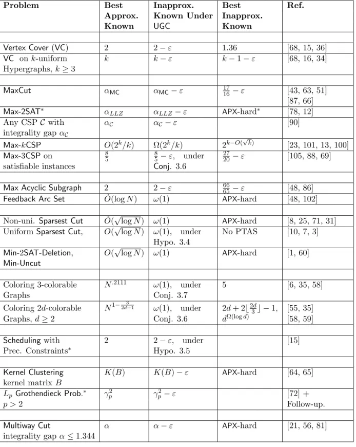
The main motivation behind formulating the UGC is to prove inapproximability results for NP -complete problems for which “satisfactory” results are not available otherwise. Figure 2 shows a table of such results. For each problem, we mention the best approximation factor known, the inapproximability factor under the UGC (or its variant), and the best inapproximability result known without relying on the UGC. The list is not necessarily exhaustive, but covers most of the results the author is aware of. The problems can be roughly classified into two categories: problems for which a constant approximation is known and the goal is to characterize the exact approximation threshold (e.g. MaxCut), and those for which the known approximation is super-constant, and the goal is to prove a super-constant inapproximability result (e.g. Min-2SAT-Deletion). Majority of these inapproximability results can be proved in the framework described in Theorem 2.6. We present a complete reduction fromGapUG toGapMin-2SAT-Deletionas an illustration. We refer to the author’s recent article [62] for a more detailed survey of such reductions.
4.1 Inapproximability of the Min-2SAT-Deletion Problem
In this section, we give a sketch of a reduction from the Unique Game problem to the Min-2 SAT-Deletion problem [60] as one illustration of the UGC-based inapproximability results. An instance of the Min-2SAT-Deletion problem is a 2SAT formula φ and OPT(φ) is defined as the minimum fraction of clauses that need to be deleted from φto make it satisfiable.
Theorem 4.1 Let 12 < c < 1 be a fixed constant. Then, for every sufficiently small constant
ε > 0, there exists a constant δ > 0 and a polynomial time reduction that maps an instance
U(G(V, E),[n],{πe|e∈E}) of theUnique Game problem to a 2SAT formula φ such that:
• (YES Case:) If OPT(U)≥1−ε, then OPT(φ)≤O(ε).
• (NO Case:) If OPT(U)≤δ, then OPT(φ)≥Ω(εc).
We actually give a reduction from the Unique Game problem to a boolean 2-CSP where the constraints are of the form x = y for boolean literals x and y. The constraints can then be converted to 2SAT clauses since x=y is equivalent to two clauses x∨y and x∨y. It is easier to view the reduction as a PCP where the verifier reads two bits from a proof and accepts if and only if the two bits are equal (or unequal, as is pre-determined). The 2-CSP can then be written down by letting the bits in the proof as boolean variables and the tests of the verifier as the constraints of the 2-CSP. In the YES Case, there is a proof that the verifier accepts with probability 1−O(ε) whereas in the NO Case, every proof is accepted with probability at most 1−Ω(εc). In terms of the 2-CSP, this means that in the YES Case, it suffices to delete O(ε) fraction of the constraints to make the 2-CSP satisfiable, and in the NO Case, one needs to delete at least Ω(εc) fraction of the constraints. An important ingredient in the PCP analysis is the Bourgain’s Noise-Sensitivity Theorem that is stated in Section 6.2 as Theorem 6.2.
The PCP construction is rather straightforward. The verifier is given a Unique Game instance
U(G(V, E),[n],{πe|e∈ E}). She expects the proof to contain, for every v ∈ V, the long code of the label ofv in a supposed labeling L:V 7→[n]. In words, for every v∈V, if L(v) =i0, then the
proof is supposed to contain the truth-table of the dictatorship function of co-ordinate i0. Each of
these functions is assumed to satisfy f(−x) =−f(x) and hence balanced. This is enforced by the standard “folding” trick: we force the proof to contain only one of the bits f(x) or f(−x) and let the other bit to be its negation.
Problem Best Inapprox. Best Ref.
Approx. Known Under Inapprox.
Known UGC Known
Vertex Cover(VC) 2 2−ε 1.36 [68, 15, 36]
VC on k-uniform k k−ε k−1−ε [68, 16, 34]
Hypergraphs,k≥3
MaxCut αMC αMC−ε 1716−ε [43, 63, 51]
[87, 66]
Max-2SAT∗ αLLZ αLLZ−ε APX-hard∗ [78, 12]
Any CSPC with αC αC−ε [90]
integrality gapαC
Max-kCSP O(2k/k) Ω(2k/k) 2k−O(
√
k) [23, 101, 13, 100]
Max-3CSPon 85 85−ε, under 2720−ε [105, 88, 69]
satisfiable instances Conj. 3.6
Max Acyclic Subgraph 2 2−ε 6665−ε [48, 86]
Feedback Arc Set O˜(logN) ω(1) APX-hard [48, 102] Non-uni. Sparsest Cut O˜(√logN) ω(1) APX-hard [8, 25, 71, 31] UniformSparsest Cut, O(√logN) ω(1), under No PTAS [10, 7, 3]
Hypo. 3.4
Min-2SAT-Deletion, O(√logN) ω(1) APX-hard [1, 60]
Min-Uncut
Coloring 3-colorable N.2111 ω(1), under 5 [6, 35, 58]
Graphs Conj. 3.7
Coloring 2d-colorable N1−2d3+1 ω(1), under 2d+ 2b2d
3 c −1, [55, 35]
Graphs,d≥2 Conj. 3.6 dΩ(logd) [58, 59]
Scheduling with 2 2−ε, under [15]
Prec. Constraints∗ Hypo. 3.5
Kernel Clustering K(B) K(B)−ε APX-hard [64, 65] kernel matrixB
Lp Grothendieck Prob.∗ γp2 γp2−ε [72] +
p >2 Follow-up.
Multiway Cut α α−ε APX-hard [21, 56, 81]
integrality gapα≤1.344
Figure 2: (In)approximability Results for Some Optimization Problems
∗ α
LLZ is the believed approximation ratio of Lewinet al’s SDP algorithm [78].
∗ APX-hard means NP-hard to approximate within some factor strictly larger than 1. ∗ Minimizing weighted completion time with precedence constraints.
∗ K(B) is a geometric parameter associated with matrixB. ∗ γ
p is thepth norm of a standard Gaussian variable. 13
The PCP Test
• Pick a random edge (v, w)∈E along with the bijectionπ=πe: [n]7→[n] associated with it. Letfv and fw be the supposed long codes corresponding tov and w respectively.
• Letx∈ {−1,1}nbe a random input and y∈ {−1,1}n be obtained by flipping every bit ofx with probability ε >0 independently.
• Do each of these two tests with probability 12 each: accept if fv(x) = fv(y) or fv(x) =
gw(π(x)), whereπ(x) := (xπ(1), . . . , xπ(n)).
YES Case: Assume the Unique Game instance has a labeling that satisfies 1−ε fraction of the edges. Take this labeling and encode each label with the corresponding dictatorship function. Since the ε-noise sensitivty of a dictatorship function is exactly ε, the test fv(x) =fv(y) accepts with probability 1−ε. For 1−εfraction of the edges, the labeling satisfies the edge, i.e. fv and
fw are dictatorships of co-ordinates i and j respectively with π(i) = j. Hence fv(x) = xi and
gw(π(x)) = (π(x))j =xπ(j) =xi, and hence the test fv(x) =gw(π(x)) accepts with probability 1. Overall, the verifier accepts with probability 1−O(ε).
NO Case: Assume for the sake of contradiction that the verifier accepts with probability at least 1− εc
200. We will construct a labeling to the Unique Game instance that satisfies more than a δ
fraction of its edges, giving a contradiction. Towards this end, first observe that by an averaging argument, it must be the case that for 99% of the vertices v ∈V, the test fv(x) =fv(y) accepts with probability at least 1−εc. Sincefv is a balanced function, applying Bourgain’s Theorem 6.2, we conclude that fv is close to a function that depends only on K := 2O(1/ε
2)
co-ordinates. Let this set of co-ordinates beSv ⊆[n],|Sv| ≤K. For the ease of argument, assume that this holds for every v ∈ V and moreover that fv depends precisely on the co-ordinates in Sv. Now consider an edge (v, w)∈E. We claim that for 99% of edges, the setsπ(Sv) andSw intersect. This is because, otherwise, the functions fv and fw depend on disjoint sets of co-ordinates (after the bijection π is applied) and therefore the testfv(x) =fw(π(x)) fails with constant probability. Finally, consider a labeling that assigns to eachv∈V, a random label from the setSv. It follows that for 99% of the edges (v, w) ∈E, the sets π(Sv) andSw intersect and hence a matching pair of labels is assigned tov and wwith probability at least K1. We choose δ K1 beforehand to reach a contradiction.
4.2 Raghavendra’s Result
A beautiful result of Raghavendra [90] shows that for every CSP C, the integrality gap αC for a
natural SDP relaxation is same as the inapproximability threshold for the CSP, modulo theUnique Games Conjecture. This is a duality type result showing that the SDP relaxation, while giving an algorithm with approximation ratio αC, also leads to an inherent limitation: it prevents every
efficient algorithm from achieving a strictly better approximation ratio.
A k-ary CSP C is defined by a collection of finitely many predicates P : {0,1}k 7→ {0,1}. By abuse of notation, we let C denote this collection of predicates as well. An instance of the CSP is specified as I(V, E,{Pe|e ∈ E}): V = {x1, . . . , xN} is a set of boolean variables and E is a collection of constraints, each being a size k subset of V. A constraint e ∈ E is denoted as
e= (xe1, . . . , xek), ei ∈[N], with a specific order on the variables, and has an associated predicate
Pe∈ C. An assignment is a mapρ:V 7→ {0,1}. An assignment ρ satisfies a constrainte if
LetOPT(I) denote the maximum fraction of constraints satisfied by any assignment. Raghavendra studies a natural SDP relaxation for the CSP that we do not describe here. LetSDP(I) denote the optimum of the SDP relxation, and define the integrality gap αC as:
αC := sup
I
SDP(I)
OPT(I),
where the supremum is taken over all instances. Clearly, OPT(I) ≤ SDP(I) ≤ αC ·OPT(I), and
hence the SDP gives an αC approximation to the CSP.8 The formal statement of Raghavendra’s
result is:
Theorem 4.2 ([90]) Suppose there is an instance I∗ of the CSP C such that SDP(I∗) ≥ c and
OPT(I∗)≤s. Then for every γ >0, there exist ε, δ >0, and a polynomial time reduction from an
Unique Game instance to an instance I of the CSP such that:
• (YES Case:) If OPT(U)≥1−ε, then OPT(I)≥c−γ.
• (NO Case:) If OPT(U)≤δ, then OPT(I)≤s+γ.
In particular, assuming the UGC, it is NP-hard to approximate the CSP within any factor strictly less than αC.
Note that the theorem turns an integrality gap to an inapproximability gap. Roughly speaking, the idea is to use the SDP gap instance to construct a dictatorship test and then combine the test (as usual) with the Unique Game instance. The analysis of the dictatorship test relies crucially on a powerful version of the invariance principle by Mossel [82] (see Section 6.4 for a more detailed description of the invariance principle).
The result of Khot et al [63] shows that assuming the UGC, it is NP-hard to approximate
MaxCutwithin any factor strictly less than αMC, the integrality gap of the Goemans-Williamson’s
SDP. The result, in hindsight, can be interpreted as turning the Feige-Schechtman integrality gap instance into an inapproximability result. However, the result relied on explicitly “knowing” the integrality gap instance. Raghavendra’s result is a generalization of [63] to every CSP. For a general CSP, the integrality gap is not explicitly known, but Raghavendra circumvents the need to know it explicitly.
Raghavendra’s result is more general: it applies to CSPs with boolean alphabet, with non-negative real valued “pay-off functions” rather than predicates, and in some restricted cases, even with possibly negative pay-offs. As a concrete example, Raghavendra and Steurer [93] show that for the Grothendieck’s Problem, even though the integrality gapKG (= the famous Grothendieck’s constant) is not known, we do know, moduloUGC, that it isNP-hard to approximate Grothendieck’s Problem within any factor strictly less thanKG. Manokaranet al[81] show how to translate linear programming integrality gap to an inapproximability gap, specifically for the Multiway Cut and related problems.
5
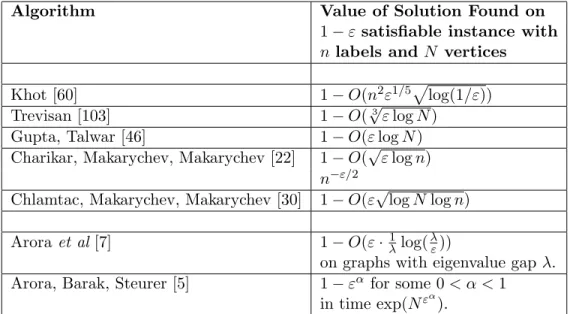
Algorithms
The UGC states that given an instance of the Unique Game problem that is 1−ε satisfiable, it is NP-hard to find an assignment that satisfies δ fraction of the constraints when the number of
8
The SDP gives the approximatevalueof the solution. Raghavendra and Steurer [91] also show how to round the solution and find an actual assignment with approximation ratio arbitrarily close toαC.
Algorithm Value of Solution Found on 1−εsatisfiable instance with
nlabels andN vertices
Khot [60] 1−O(n2ε1/5plog(1/ε))
Trevisan [103] 1−O(√3εlogN)
Gupta, Talwar [46] 1−O(εlogN)
Charikar, Makarychev, Makarychev [22] 1−O(√εlogn)
n−ε/2
Chlamtac, Makarychev, Makarychev [30] 1−O(ε√logNlogn)
Arora et al [7] 1−O(ε·1
λlog( λ ε))
on graphs with eigenvalue gapλ. Arora, Barak, Steurer [5] 1−εα for some 0< α <1
in time exp(Nεα). Figure 3: Algorithms for theUnique Game Problem
labelsn=n(ε, δ) is a sufficiently large constant. Therefore agood enoughalgorithm for theUnique Game problem would disprove the conjecture. Figure 3 summarizes the algorithmic results so far: given an 1−ε satisfiable instance with N vertices and n labels, the second column specifies the fraction of the constraints satisfied by an assignment found by the algorithm.
We note that the algorithmic results fall short of disproving the UGC: In [60, 22], for constant
ε > 0, the algorithm does not work when n is sufficiently large but still constant (which the conjecture allows). In [103, 46, 30], the algorithm works only whenεis a sub-constant function of the instance size N whereas the conjecture is about constant ε > 0. In [7], the algorithm works only when the graph is a (mild) expander. In [5], the algorithm runs in sub-exponential time. On the other hand, these algorithms can be interpreted as meaningful trade-offs between quantitative parameters if the UGCwere true: one must have n 21/ε [22], the graph cannot even be a mild expander and in particular its eigenvalue gap must satisfy λε[7], and the presumed reduction from 3SAT to the GapUG problem must blow up the instance size by a polynomial factor where the exponent of the polynomial grows as ε → 0 [5]. Moreover, the conjecture cannot hold for
ε √ 1
logN [103, 46, 30]; this places a limitation on the inapproximability factor that can be proved for problems such as Sparsest Cut, where one is interested in the inapproximability factor as a function of the input size.
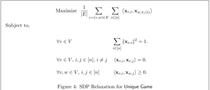
We present a very brief overview of some of these algorithms. With the exception of [46, 5], all algorithms depend on a natural SDP relaxation for the Unique Gameproblem shown in Figure 4. We skip the minor differences in the SDP formulations used in different papers. The SDP relaxation was introduced and studied by Feige and Lovasz [39] in the context of parallel repetition (see Section 7).
For a Unique Game instance U(G(V, E),[n],{πe|e ∈ E}), one can write a quadratic integer program in the following manner: for every v ∈ V and i∈ [n], letxv,i be a {0,1}-valued integer variable such that xv,i = 1 if and only if L(v) =ifor some supposed labelingL:V 7→[n]. Clearly one can write down the constraints thatPn
Maximize 1
|E| X
e=(v,w)∈E
X
i∈[n]
xv,i,xw,πe(i)
Subject to,
∀v∈V X
i∈[n]
kxv,ik2= 1.
∀v∈V,i, j ∈[n], i6=j hxv,i,xv,ji= 0.
∀v, w∈V,i, j∈[n] hxv,i,xw,ji ≥0. Figure 4: SDP Relaxation for Unique Game
The fraction of constraints satisfied is: 1
|E| X
e=(v,w)∈E
X
i∈[n]
xv,i·xw,πe(i).
The SDP relaxation in Figure 4 is obtained by relaxing integer variables xv,i to vectors xv,i and replacing integer products by vector inner products.
For simplicity of exposition, let us restrict ourselves to the case of linear unique games, as in the definition preceding Conjecture 3.2. Such games are symmetric in the following sense: if
L :V 7→ [n] is a labeling, then for any constant c ∈ Zn, the labeling L0(v) =L(v) +c(mod n) is another labeling that satisfies exactly the same set of edges. This symmetry allows us to add more constraints to the SDP and ensure that in the SDP solution,∀v ∈V,∀i∈[n], kxv,ik= √1n. Thus, for every v ∈V, we have an orthonormal tuple of vectors{xv,i}ni=1 up to a normalizing factor of
1 √
n. Assume that we have aUnique Gameinstance that is 1−εsatisfiable. Thus, the SDP optimum is also at least 1−ε, and it is an average over the contribution over all edges. For simplicity of exposition, let us also assume that the contribution over every edgee= (v, w) is at least 1−ε. For linear games, by symmetry, this ensures that ∀i∈[n],
xv,i, xw,πe(i)
≥(1−ε)· 1
n.
5.1 Khot’s [60] and Charikar, Makarychev, Makarychev’s [22] Algorithms
Assume that the vectors are inRd and consider the following natural rounding procedure:
SDP Rounding:
• Pick a random unit vectorrinRd.
• For eachv∈V, define its label to be L(v) =i0 where i0 = arg max
i∈[n] |hr,xv,ii|.
The analysis works on edge by edge basis. Fix any edge e = (v, w). We have two tuples
{xv,i}ni=1 and {xw,πe(i)} n
i=1 for vertices v and w respectively. As we said before, we will make
simplifying assumptions that ∀i, j,kxv,ik = kxw,jk = √1n and that
xv,i, xw,πe(i)
≥ (1−ε)· n1.
Thus the two tuples are very “close” and it is intuitively clear that for a random vector r, the vectors in the two tuples that maximize the inner product withrare likely to be a “matching” pair of vectors. Formally, we need to analyze the probability that the rounding algorithm “succeeds” on the edge, i.e. the probability that it assigns a label i0 to v and the matching label πe(i0) to w. In [60], a rather crude estimate is given, whereas Charikar, Makarychev, and Makarychev [22] give the optimal 1−O(√εlogn) bound on this probability. For a general unique game (i.e. not necessarily linear), in an SDP solution, the vectors {xv,i}ni=1 need not have equal norms. In this
case, the rounding procedure in [22] is considerably more sophisticated and the analysis technically challenging. A rough intuition is that {kxv,ik2}ni=1 can be thought of as a probability distribution
on the labels for a vertex v and the rounding procedure should pick a label i with probability
kxv,ik2, simultaneously for all vertices in a coordinated manner. The result is applicable when
ε log1n. In the regime when ε log1n, the authors of [22] give an alternate rounding procedure that satisfies n−ε/2 fraction of the constraints.
5.2 Trevisan’s Algorithm [103]
Trevisan [103] presents a simple and elegant algorithm that first partitions theUnique Gamegraph into components with low diameter and then on each component, finds a good labeling. The SDP relaxation is augmented with the so-called triangle inequality constraints that we omit from this discussion. Assume, again for simplicity, that theUnique Gameinstance is 1−εsatisfiable and every edge contributes at least 1−ε towards the SDP objective. We first apply a graph decomposition theorem of Leighton and Rao [77] that removes ε fraction of the edges so that each connected component has diameter at most O(logN/ε). We “give up” on the edges that are removed and find a good labeling for each of the components separately. On each component, fix one vertexv
and consider the vectors {xv,i}ni=1. Choose the label of v to be i0 ∈ [n] with probability kxv,i0k
2.
Once the label i0 forv is fixed, for every other vertex w in the component, define its label to be j∈[n] that minimizeskxw,j−xv,i0k
2. Intuitively, since the component has bounded diameter, the
label at one vertex more or less determines labels of all vertices in the component (e.g. consider the extreme case when a component is a clique. In this case, the vector tuples for all the vertices in the component are pairwise close to each other). The actual analysis is fairly simple using the triangle inequality constraints.
5.3 Arora et al’s Algorithm [7]
This algorithm is again based on the SDP relaxation and works as long as the graph is a mild expander. Let us again make the simplifying assumptions that ∀v ∈ V,∀i,kxv,ik = √1n and that for every edge e= (v, w) ∈E, xv,i, xw,πe(i)
≥(1−ε)· 1
n. A useful observation is that one can define a single unit vector xv := n3/2 ·Pni=1x⊗4v,i that captures the behavior of the entire tuple in the following sense: for every edge (v, w), we know that the tuples {xv,i}ni=1 and {xw,πe(i)}
n i=1
are close and therefore it holds that hxv,xwi ≥ 1−O(ε). Now consider the random hyperplane cut on the set of vectors S := {xv | v ∈ V}. Each edge (v, w) is cut with probability O(
√
ε) since hxv,xwi ≥ 1−O(ε). If the set S were “well-spread” on the unit sphere, then the cut will be roughly balanced. This would imply that the Unique Game graph has a roughly balanced cut that cutsO(√ε) fraction of the constraints, contradicting the assumption that the graph is a mild expander. Therefore, the setS cannot be well-spread, i.e. most vectors inSare confined to a small
neighborhood on the unit sphere. This implies, in turn, that the tuples {xv,i}ni=1 for almost all v ∈V are pairwise close to each other (we already know that the tuples are close whenever there is an edge/constraint between them, but now this holds irrespective of it) and this easily yields a good global labeling. The expansion requirement in [7] is stated in terms of eigenvalue gap, but as we indicated, it also works w.r.t. edge expansion. This was also observed and the result somewhat improved in [80].
5.4 Arora, Barak, Steurer’s Algorithm [5]
For some 0< α < 1, Arora, Barak, and Steurer [5] give an algorithm that runs in time exp(Nεα) and finds a labeling that satisfies 1−εα fraction of the edges. The algorithm is motivated by the connection between Unique Game problem and the Small Set Expansion problem mentioned below. The algorithm is based on the approach of Naor [84] and given a graph G(V, E) whose stochastic matrix has at least M eigenvalues larger than 1−ε, the algorithm finds a set S ⊆ V
of size Npoly(ε)/M with expansion at most poly(ε). Ideas of Kolla [74] are also used who gives a method for solving unique games on graphs with few large eigenvalues. The author just received the manuscript of [5] at the time of writing this article, so prefers to include only this brief description.
5.5 The Small Set Expansion Problem:
Raghavendra and Steurer [94] give a reduction from theSmall Set Expansionproblem to theUnique Game problem. Whereas we have several reductions from theUnique Game problem to other opti-mization problems, this is the first reduction in the other direction. It would indeed be interesting if some natural problem is equivalent to theUnique Gameproblem, and hence “UG-complete”. The
Small Set Expansion problem is certainly a candidate and so is theGapMaxCut1−ε, 1−b·√
ε problem as discussed in Section 7.
For a d-regular graph G(V, E) and a set S ⊆ V, define the expansion of the set S as φ(S) :=
|E(S,V\S)|
d·|S| , i.e. the fraction of edges incident onS that leave S. One could hypothesize that:
Hypothesis 5.1 For everyε >0, there exists γ >0 such that given a regular graphG(V, E), it is
NP-hard to distinguish between:
• (YES Case:) There is a set S⊆V,|S|=γ|V| such thatφ(S)≤ε.
• (NO Case:) For every set S⊆V,|S|=γ|V|, φ(S)≥1−ε.
In words, it is hard to find a small set in a graph that is somewhat non-expanding even when we are guaranteed that there exists a small set that is almost non-expanding. Raghavendra and Steurer [94] show that this conjecture implies the Unique Games Conjecture.
Theorem 5.2 ([94]) Hypothesis 5.1 implies Conjecture 2.5 (UGC).
We give some intuition here why theUGCis related to the small set expansion problem. Suppose
U(G(V, E),[n],{πe|e∈E}) is an instance ofUnique Game. Consider the following graphG0(V0, E0):
V0 :=V ×[n] and ((v, i),(w, j))∈E0 if and only if (v, w) =e∈E and πe(i) =j.
In words, G0 is obtained by replacing every vertex of G by a block of n vertices and every bijective constraint of theUnique Gameinstance is replaced by a matching between the two blocks. It is easy to see that if the Unique Game instance has a labeling L : V 7→ [n] that satisfies 1−ε
fraction of the constraints, then the set S := {(v, L(v))|v ∈V} ⊆ V0 is a subset with relative size
1
n and expansion at most ε. Thus a good labeling to the Unique Game instance corresponds to a small non-expanding set in G0.
6
Discrete Fourier Analysis
In this Section, we give a brief overview of Fourier analytic theorems that have found applications to inapproximability. We refer to [62] for a more detailed exposition.
6.1 Friedgut’s Theorem
Theorem 6.1 ([42]) Let k, γ >0 and let f :{−1,1}n 7→ {−1,1} be a boolean function with total influence (a.k.a. average sensitivity) at most k. Then there exists a boolean functiong that agrees with f on 1−γ fraction of inputs and depends on at most 2O(k/γ) co-ordinates.
Friedgut’s Theorem was used by Dinur and Safra [36] to prove 1.36 inapproximability result for theVertex Coverproblem. Their paper, and to a lesser extent the application of Bourgain’s Theorem in [60], were the early examples where a “special purpose” powerful Fourier analytic theorem was applied in the context of inapproximability. Friedgut’s Theorem was subsequently used to prove
UGC-based 2−ε inapproximability result for Vertex Cover [68]. A theorem of Russo [99] is also used in theVertex Coverapplications: for amonotoneboolean functionf, the probability Pr[f = 1] under ap-biased distribution is an increasing, differentiable function ofp, and its derivative equals the average sensitivity.9
6.2 Bourgain’s Noise-Sensitivity Theorem
Recall that for 0 < ε < 12, the ε-noise sensitivity NSε(f) is defined as the probability Pr[f(x) 6=
f(y)] where x is a uniformly random input and the input y is obtained by flipping every bit of x
independently with probability ε.
Theorem 6.2 ([20]) Let 12 < c < 1 be any fixed constant. For all sufficiently small ε > 0, if
f : {−1,1}n 7→ {−1,1} is a function with ε-noise sensitivity at most εc, then there is a boolean functiong that agrees withf on99% of the inputs and g depends only on 2O(1/ε2) co-ordinates.
Bourgain’s Theorem is tight: for c = 12, the MAJORITY function has ε-noise sensitivity θ(εc), but cannot be approximated by a function that depends on a bounded number of co-ordinates. The theorem was motivated by H˚astad’s [50] observation that such a theorem could lead to a super-constant inapproximability result for the Min-2SAT-Deletion problem. It was observed in [60] that the desired inapproximability result can indeed be proved, albeit using the Unique Games Conjecture. The theorem was subsequently used to prove a super-constant inapproximability result as well as (log logN)1/7 integrality gap result for the non-uniform Sparsest Cut problem [71]. The gap holds for a natural SDP with so-calledtriangle inequality constraintsand can be interpreted as a construction of anN-pointnegative typemetric that incurs distortion (log logN)1/7 to embed into
`1. It refuted a conjecture of Goemans and Linial [44, 79] that every negative type metric embeds
into `1 with constant distortion (which would have implied a constant factor approximation to
non-uniformSparsest Cut). These connections are further explained in Section 8.2.
6.3 Kahn, Kalai, Linal’s Theorem
Theorem 6.3 ([54]) Every (13,23)-balanced boolean functionf :{−1,1}n7→ {−1,1} has a variable whose influence is Ωlognn.
9
f is monotone if flipping any bit of an input from−1 to 1 can only change the value of the function from−1 to 1. Ap-biased distribution is a product distribution such that on each co-ordinate, Pr[xi= 1] =p.
The KKL Theorem has been used to prove a super-constant inapproximability result for the non-uniform Sparsest Cut problem by Chawla et al [25] and to construct Ω(log logN) integrality gaps for a natural SDP relaxation for the non-uniform as well as the uniform Sparsest Cutproblem [75, 33], improving on the integrality gap obtained earlier in [71].
6.4 Majority Is Stablest and Borell’s Theorem
Bourgain’s Theorem gives a lower bound of Ω(εc) on the noise sensitivity of a balanced function whose all influences are small andc > 12. TheMajority Is StablestTheorem [83] gives an exact lower bound, namely 1πarccos(1−2ε), which coincides with theε-noise sensitivity of then-bitMAJORITY
function asn→ ∞. TheMajority Is StablestTheorem was conjectured in [63] and used to prove that the approximation factor achieved by Goemans and Williamson’s algorithm forMaxCutis optimal. Theorem 6.4 (Mossel, O’Donnell, Oleszkiewicz [83]) Fix 0< ε < 12. Let f :{−1,1}n 7→ {−1,1} be a balanced function with all its influences at most η. then
NSε(f)≥ 1
π arccos(1−2ε)−δ,
where δ →0 as η→0.
We present a sketch of the proof as it demonstrates the connection to an isoperimetric problem in geometry and its solution by Borell [19]. The proof involves an application of the invariance principle, also studied by Rotar [98] and Chatterjee [24], with Mossel’s [82] results being the state of the art. Here is a rough statement of the invariance principle:
Invariance Principle [98, 83, 24, 82]: Suppose f is a low degree multi-linear polynomial in
n variables and all its variables have small influence. Then the distribution of the values of f is nearly identical when the input is a uniform random point from {−1,1}n or a random point from
Rn with standard Gaussian measure.
The invariance principle allows us to translate the noise sensitivity problem on boolean hyper-cube to a similar problem in the Gaussian space and the latter problem has already been solved by Borell! Towards this end, letf :{−1,1}n 7→ {−1,1} be a balanced boolean function whose all influences are at most η. We intend to lower bound its ε-noise sensitivity. We know that f has a representation as a multi-linear polynomial, namely its Fourier expansion:
f(x) = X S⊆[n]
b
f(S)Y i∈S
xi ∀x∈ {−1,1}n.
Letf∗ :Rn7→Rbe a function that has the same representation as a multi-linear polynomial as f:
f∗(x∗) = X S⊆[n]
b
f(S)Y i∈S
x∗i ∀x∗∈Rn. (1)
Assume for the time being thatf haslowdegree. Sincef has all influences small, by the invariance principle, the distributions of f(x) and f∗(x∗) are nearly identical, and let us assume them to be exactly identical for the sake of argument. This implies that E[f∗] = E[f] = 0 and since f is
boolean, so isf∗. In other words,f∗ is a partition ofRninto two sets of equal (Gaussian) measure.
The next observation is that theε-noise sensitivity off is same as theε-“Gaussian noise sensitivity” of f∗ : Rn 7→ {−1,1}. To be precise, let (x∗, y∗) be a pair of (1−2ε)-correlated n-dimensional
Gaussians, i.e. for every co-ordinatei, (x∗i, yi∗) are (1−2ε)-correlated standard Gaussians. One way 21
to generate such a pair is to pick two independent standard n-dimensional Gaussians x∗ and z∗, and let y∗ = (1−2ε)x∗+p1−(1−2ε)2z∗, and thus one can think ofy∗ as a small perturbation
of x∗. Let theε-noise sensitivity of a function f∗:Rn7→ {−1,1}be defined as:
NSε(f∗) := Prx∗∼
1−2εy∗[f
∗(x∗)6=f∗(y∗)].
When f∗ is a multi-linear polynomial as in (1), it is easily observed that
NSε(f∗) = 1 2 −
1 2
X
S⊆[n]
b
f(S)2(1−2ε)|S|.
But this expression is same as the ε-noise sensitivity of the boolean function f and thus NSε(f) =
NSε(f∗) and Theorem 6.4 follows from Borell’s result that lower boundsNSε(f∗). The parameter
δ in the statement of Theorem 6.4 accounts for additive errors involved at multiple places during the argument. Also, we need to make sure that f is a low degree function in order to apply the invariance principle; this is handled bysmoothening the function beforehand; we omit the details. Theorem 6.5 ([19]) If f∗ :Rn7→ {−1,1} is a measurable function with E[f∗] = 0, then
NSε(f∗)≥NSε(HALF SPACE) = 1
π arccos(1−2ε),
where HALF-SPACE is the partition of Rn by a hyperplane through origin.
6.5 It Ain’t Over Till It’s Over Theorem
For a set of co-ordinates S⊆ {1, . . . , n}and a string x∈ {−1,1}n, a sub-cubeC
S,x corresponds to the set of all inputs that agree with xoutside of S, i.e.
CS,x :={z |z∈ {−1,1}n, ∀i6∈S, zi=xi}.
A random sub-cubeCS,xof dimensionεnis picked by selecting a random setS⊆ {1, . . . , n},|S|=εn and a random string x. For a (roughly) balanced function f, consider the probability that f is constant on a random sub-cube of dimension εn. The dictatorship function passes the test with probability 1−ε whereas it can be shown that if f has all its influences small, then f passes the test with small probability. It follows from the It Ain’t Over Till It’s Over Theorem of Mossel et al[83]. The theorem is in fact stronger: iff has all influences small, then for almost all sub-cubes
C, not only thatf is non-constant onC, butf takes both the values{−1,1}on a constant fraction of points in C. A formal statement appears below:
Theorem 6.6 ([83]) For every ε, δ >0, there exist γ, η >0 such that iff :{−1,1}n7→ {−1,1} is a (13,23) balanced function with all influences at most η, then
PrC
h
E[f(x)|x∈C]
≥1−γ i
≤ δ,
where C is a randomεn-dimensional sub-cube.
The theorem is proved using the invariance principle. Bansal and Khot [15] give an alternate simple proof without using the invariance principle (the random sub-cube test is proposed therein), but the conclusion is only that f is non-constant on almost every sub-cube (which suffices for their application). The random sub-cube test qualifies as a one free bit Long Code test, with completeness close to 1 and soundness close to zero. Via a connection between PCPs and the
Independent Set problem, it implies that given an N-vertex graph with two disjoint independent sets of size (12 −ε)N each, it is NP-hard to find an independent set of sizeδN, modulo UGC[15].