Charles University
Faculty of Mathematics and Physics
Mgr. Daniel Pr˚
uˇsa
Two-dimensional Languages
Doctoral Thesis
Supervisor: Martin Pl´
atek, CSc.
Acknowledgements
The results presented in this thesis were achieved during the years 1998–2004. Many of them were achieved within the framework of grant projects. They include Grant-No. 201/02/1456 (The Grant Agency of the Czech Republic) and Grant-No. 300/2002/A-INF/MFF (The Grant Agency of Charles University, Prague).
I would like to gratefully thank my supervisor Martin Pl´atek, CSc. for his valuable support he provided me during writing the thesis.
Contents
1 Introduction 6
1.1 Studied Two-dimensional Formal Models . . . 6
1.2 Goals . . . 9
1.3 Achieved Results . . . 10
1.4 Notation . . . 11
2 Theory of Picture Languages 12 2.1 Pictures, Picture Languages . . . 12
2.2 Two-dimensional Turing Machines . . . 14
2.3 Notes on Computational Techniques . . . 16
3 Two-dimensional Finite-state Automata 19 3.1 Finite-state Automaton . . . 19
3.2 Finite-state Automata over One-symbol Alphabet . . . 20
3.3 Simulation of Finite-state Automata by Deterministic Turing Ma-chines . . . 25
4 Time Complexity in Two Dimensions 37 4.1 N P2d-completeness . . . . 37
4.2 Recognition of Palindromes . . . 42
4.3 Crossing Sequences . . . 45
4.4 Lower Bounds on Time Complexity . . . 47
5 Two-dimensional On-line Tessellation Automata 49 5.1 Properties ofOT A . . . 49
5.2 Simulation of Cellular Automata . . . 51
6 Two-dimensional Forgetting Automata 59 6.1 Technique Allowing to Store Information in Blocks . . . 59
6.2 Forgetting Automata andN P2d-completeness . . . . 63
7 Grammars with Productions in Context-free Form 67 7.1 Introduction into Two-dimensional Context-free Grammars . . . 67
7.2 CF P Grammars, Derivation Trees . . . 71
7.3 L(CF P G) in Hierarchy of Classes . . . 74
7.4 Restrictions on Size of Productions’ Right-hand Sides . . . 84
7.5 Sentential Forms . . . 87
7.6 CF P Grammars over One-symbol Alphabet, Pumping Lemma . 91 7.7 Closure Properties . . . 96
7.8 Emptiness Problem . . . 101 7.9 Comparison to Other Generalizations of Context-free Languages 107
Chapter 1
Introduction
This thesis presents results on the theory of two-dimensional languages. The theory studies generalizations of formal languages to two dimensions. These generalizations can be done in many different ways. Automata working over a two-dimensional tape were firstly introduced by M. Blum and C. Hewitt in 1967. Since then, several formal models recognizing or generating two-dimensional objects have been proposed in the literature. All these approaches were initially motivated by problems arising in the framework of pattern recognition and image processing. Two-dimensional patterns also appear in studies concerning cellular automata and some other models of parallel computing.
The most common two-dimensional object is apicturewhich is a rectangular array of symbols taken from a finite alphabet. We restrict ourselves to the study of languages build from such objects. These languages are calledpicture languages.
1.1
Studied Two-dimensional Formal Models
We give the informal description of the models studied in this thesis. Two-dimensional Turing machine
A Turing machine provided by a dimensional tape (which is a two-dimensional array of fields infinite in both directions) with the capability to move the head in four directions – left, right, up and down – is called a two-dimensional Turing machine. Such a machine can be used to recognize picture languages. In the initial configuration, an input picture is stored in the tape. The head scans typically the upper-left corner. The fields of the tape not con-taining a symbol of the input are filled by thebackground symbol # (it is also known as theblank symbol). The computation over the input is an analogy to computations of the model with one-dimensional tape.
The two-dimensional Turing machine can be considered as the most general two-dimensional recognizing device. The class of languages recognizable by two-dimensional Turing machines is an analogy to 0 languages of the Chomsky hierarchy (recursively enumerable languages). The origin of the model dates to late sixties of the twentieth century, when the basics of the theory were formed.
Two-dimensional finite-state automaton
We say that a two-dimensional Turing machine isbounded if the machine does not move the head outside the area of the input. To be more precise, the head is allowed to leave the area in a step but whenever this situation occurs, it does not rewrite the scanned background symbol and it has to be moved back in the next step.
Each bounded two-dimensional Turing machine that never rewrites any sym-bol of the tape is called a two-dimensional finite-state automaton. It is also known as a four-way automaton. Similarly as in the case of two-dimensional Turing machines, two-dimensional finite-state automata were proposed in be-ginnings of the theory of two-dimensional languages and, since then, their prop-erties have been widely studied. The different topology of pictures (compar-ing to str(compar-ings) has an impact on results that differ to results known from the one-dimensional theory. It can be demonstrated even on the two-dimensional finite-state automata, which, in fact, can be considered as one of the simplest recognizing devices. For example, non-deterministic two-dimensional finite-state automata are more powerful than deterministic two-dimensional finite-state au-tomata.
Since two-dimensional finite-state automata are the natural extension of one-dimensional two-way automata, the formed class of picture languages recogniz-able by them is the natural candidate for the generalization of the class of regular languages.
Two-dimensional forgetting automaton
The one-dimensional forgetting automaton is a bounded Turing machine that uses a doubly linked list of fields rather than the usual tape. The automaton can erase the content of a scanned field by the special erase symbol or it can completely delete the scanned field from the list. Except these two operations, no additional rewriting of symbols in fields are allowed. One-dimensional for-getting automata were studied by P. Jancar, F. Mraz and M. Platek, e.g. in [7], where the taxonomy of forgetting automata is given, or in [8], where forgetting automata are used to characterize context-free languages.
The two-dimensional forgetting automaton is a bounded two-dimensional Turing machine that can again erase the scanned field, but it cannot delete it. It would be problematic to define this operation, since the deletion of a field from an array breaks the two-dimensional topology. These automata were studied by P. Foltyn [1] and P. Jiricka [9].
Two-dimensional on-line tessellation automaton
The two-dimensional on-line tessellation automaton was introduced by K. Inoue and A. Nakamura [5] in 1977. It is a kind of bounded two-dimensional cellular automaton. In comparison with the cellular automata, computations are per-formed in a restricted way – cells do not make transitions at every time-step, but rather a ”transition wave” passes once diagonally across them. Each cell changes its state depending on two neighbors – the top one and the left one. The result of a computation is determined by the state the bottom-right cell finishes in.
D. Giammarresi and A. Restivo present the class of languages recognizable by this model as the ground level class of the two-dimensional theory ([2]), prior to languages recognizable by two-dimensional finite-state automata. They argue that the class proposed by them fulfills more natural requirements on such a generalization. Moreover, it is possible to use several formalisms to define the class: except tessellation automata, they include tiling systems or monadic second order logic, thus the definition is robust as in the case of regular languages.
Two-dimensional grammars with productions in context-free form The basic variant of two-dimensional grammars with productions in context-free form was introduced by M. I. Schlesinger and V. Hlavac [22] and also by O. Matz [13]. Schlesinger and Hlavac present the grammars as a tool that can be used in the area of syntactic methods for pattern recognition. Productions of these grammars are of the following types:
1) N →a 2) N →A 3) N → A B 4) N→ AB
whereA,B,N are non-terminals andais a terminal. Pictures generated by a non-terminal are defined using recurrent rules:
• For each production of type 1),N generatesa.
• For each production of type 2), if AgeneratesP, thenN generatesP as well.
• For each production of type 3) (resp. 4)), ifAgeneratesP1 andB
gener-ates P2, where the numbers of rows (resp. columns) ofP1 andP2 equal,
then the concatenation of P1andP2, whereP2 is placed after (resp.
bel-low)P1, is generated byN.
In [9], P. Jiricka works with an extended form of productions. Right-hand sides consist of a general matrix of terminals and non-terminals.
All the mentioned authors call the grammars two-dimensional context-free grammars. We will see that many properties of the raised class are not analogous to the properties of one-dimensional context-free languages. That is the reason why we prefer the term grammars with productions in context-free form.
The following table shows abbreviations we use for the models. Abbreviation Recognizing device, resp. generative system
TM two-dimensional Turing machine
FSA two-dimensional finite-state automaton
OTA two-dimensional on-line tessellation automaton
FA two-dimensional forgetting automaton
CFPG grammar with productions in context-free form Furthermore, for each listed computational model, to denote the determin-istic variant of the model we use the correspondent abbreviation prefixed byD
(i.e., we writeDT M,DF SA,DOT AandDF A). The class of languages recog-nizable, resp. generated by a modelM is denoted byL(M) (e.g. L(F SA)).
The chosen abbreviations do not reflect two-dimensionality of the models. In fact, T M, F SA and F A match the commonly used abbreviation for one-dimensional models. However, this fact should not lead to any confusions. We will refer one-dimensional models rarely and whenever we do it, we will empha-size it explicitly.
1.2
Goals
In the presented work, we focus mainly on two areas.
• Firstly, we study relationships among the two-dimensional formal models listed before.
• Secondly, we also contribute to the question of possibilities to generalize the Chomsky hierarchy to two dimensions.
As for the first goal, we are interested in the comparison of generative, resp. recognitive power of models, mutual simulations among them, questions related to time complexity. If possible, we would also like to develop general techniques or ideas of proof (e.g. the technique allowing to prove that a language is not included inL(CF P G)).
When speaking about a generalization, we have on mind the class of picture languages that fulfills some natural expectations. Let us assume to look for a generalization of regular languages. Then, as a primary requirement, we expect that, in some sense, the generalization includes regular languages. To be more precise, we mean if the two-dimensional generalization is restricted to languages containing pictures formed only of one row (resp. column), we get exactly the class of regular languages. Furthermore, we would like the mechanism defining languages in the generalized class to resemble mechanisms used to define regular languages (as finite state automata, regular grammars, etc.). In addition, we expect that the generalization inherits as many as possible properties (like closure properties) of the one-dimensional class. And finally, time complexity of recognition of languages in the class should also be important. In the case of regular languages we would expect that it is possible to decide the question of membership in time linear in number of fields of an input picture.
We have already noted that the class of languages recognizable by two-dimensional finite-state automata is the natural candidate for the generaliza-tion of regular languages. There are also some proposals of classes of picture languages generated by mechanisms resembling context-free grammars, however the properties of these classes do not fulfill the natural expectations.
We study the question whether the class of languages generated by grammars with productions in context-free form is a good generalization of one-dimensional context-free languages or not. In the mentioned literature regarding the gram-mars, there are only a few basic results on properties of the class. We would like to extend these results to have basis to make a conclusion. We will investigate the following topics:
• The comparison of L(CF P G) to the class of languages generated by the basic variant of the grammars.
• Closure properties of L(CF P G).
• Searching for a recognizing device equivalent to the grammars. We would like to propose a device based on the idea of forgetting.
• The comparison to other proposals of the generalization of context-free languages.
1.3
Achieved Results
The main results that have been achieved categorized by models are as follows:
FSA:We give a characterization of two-dimensional finite-state automata work-ing on inputs over one-symbol alphabets. We show thatL(F SA) is not closed under projection into such alphabets.
We also investigate possibilities how to simulate the automata by determin-istic bounded two-dimensional Turing machines. This result is connected to work in [10], where the simulation ofF SAby a deterministicF Ais described. The main goal is to prove the existence of such a simulation there. In our case, we rather focus on time complexity of the simulation.
OTA:We show a connection between the automata and one-dimensional cellu-lar automata. Under some circumstances, tessellation automata can simulate cellular automata. As a consequence, it gives us a generic way how to design tessellation automata recognizingN P-complete problems that are recognizable by one-dimensional cellular automata. This possibility speaks against the sug-gestion to take the class as the ground level of the two-dimensional hierarchy. Results regarding the simulation were published in [17].
FA: In [9], the technique allowing to store some information on the tape pre-serving the possibility to reconstruct the original content has been described. Using the technique, we show that forgetting automata can simulate tessellation automata as well as grammars with productions in context-free form (for every
CF P G G, there is aF Aaccepting the language generated by G).
TM: Questions related to time complexity of the recognition of pictures are studied in general. For convenience, we define the class of picture languages recognizable by two-dimensional non-deterministic Turing machines in polyno-mial time and show a relationship to the known one-dimensional variant of the class.
We also deal with lower bounds on time complexity in two dimensions. Our results are based on the generalization of so called crossing sequences and the technique related to them. It comes from [4]. Moreover, we show that a two-dimensional tape is an advantage – some one-dimensional languages can be recognized substantially faster by a Turing machine, when using the two-dimensional tape instead of the one-two-dimensional tape. These results have roots
in author’s diploma thesis ([19]), where models of parallel Turing machines work-ing over the two-dimensional tape are studied. Related results were published in [14] and [15].
CFPG: We show that L(CF P G) has many properties that do not conform the natural requirements on a generalization of context-free languages. These properties include:
• L(CF P G) is incomparable withL(F SA).
• There is no analogy to the Chomsky normal form of productions. The generative power of the grammars is dependent on size of right-hand sides of productions.
• The emptiness problem is not decidable even for languages over a one-symbol alphabet.
Next results on the class include closure properties, a kind of pumping lemma or comparisons to other proposals of the generalization of context-free languages. We have already mentioned the result regarding a relationship between gram-mars in context-free form and two-dimensional forgetting automata – each lan-guage generated by a grammar with productions in context-free form can be recognized by a two-dimensional forgetting automaton. On the other hand, the two-dimensional forgetting automata are stronger, since they can simulate two-dimensional finite-state automata. We did not succeed in finding a suitable restriction on F A’s to get a recognizing device for the class L(CF GP). At-tempts based on automata provided with a pushdown store were not successful too.
Some of the results we have listed above were published in [16] and [18].
1.4
Notation
In the thesis, we denote the set of natural numbers byN, the set of integers by
Z. Next,N+=N\ {0}.
lin :N→Nis a function such that∀n∈N: lin(n) =n. For two functions f, g:N→N, we write
• f =O(g) iff there aren0, k∈Nsuch that∀n∈Nn≥n0⇒f(n)≤k·g(n)
• f = Ω(g) iff there aren0, k∈Nsuch that∀n∈Nn≥n0⇒k·f(n)≥g(n)
• f =o(g) iff for anyk∈Nthere isn0∈Nsuch thatf(n0)≥k·g(n0)
We will also use the first notation for functions f, g : N×N→ N. In this case,f =O(g) iff there aren0, m0, k∈Nsuch that
∀n, m∈Nn≥n0∧m≥m0⇒f(m, n)≤k·g(m, n)
As for the theory of (one-dimensional) automata and formal languages, we use the standard notation and notions that can be found in [4].
Chapter 2
Theory of Picture
Languages
2.1
Pictures, Picture Languages
In this section we extend some basic definitions from the one-dimensional theory of formal languages. More details can be found in [20].
Definition 1 Apictureover a finite alphabetΣis a two-dimensional rectangu-lar array (matrix) of elements of Σ, moreover, Λ is a special picture called the
empty picture. Σ∗∗ denotes the set of all pictures over Σ. Apicture language
overΣis a subset ofΣ∗∗.
LetP∈Σ∗∗ be a picture. Then, rows(P), resp. cols(P) denotes the number
of rows, resp. columns ofP (we also call it theheight, resp. width of P). The pair rows(P)×cols(P) is called thesizeofP. We say thatP is a square picture of sizenif rows(P) = cols(P) =n. The empty picture Λ is the only picture of size 0×0. Note that there are no pictures of sizes 0×kork×0 for anyk >0. For integersi, j such that 1≤i≤rows(P), 1≤j ≤cols(P),P(i, j) denotes the symbol inP at coordinate (i, j).
Example 1 To give an example of a picture language, let Σ1 ={a, b},L be
the set consisting exactly of all square picturesP ∈Σ1∗∗, where
P(i, j) =
½
a ifi+j is an even number
b otherwise Pictures inLof sizes 1, 2, 3 and 4 follow.
a a bb a
a b a b a b a b a
a b a b b a b a a b a b b a b a
LetP1be another picture over Σ of sizem1×n1. We sayP1is asub-picture
• cx+m1−1≤mandcy+n1−1≤n
• for alli= 1, . . . , m1;j= 1, . . . , n1it holdsP1(i, j) =P(cx+i−1, cy+j−1) Let [aij]m,ndenote the matrix
a1,1 . . . a1,n ..
. . .. ...
am,1 . . . am,n
We define two binary operations – therow andcolumn concatenation. Let
A = [aij]k,l and B = [bij]m,n be non-empty pictures over Σ. The column concatenation AdB is defined iff k = m and the row concatenation AdB iff
l=n. The products of these operations are given by the following schemes:
AdB=
a11 . . . a1l b11 . . . b1n ..
. . .. ... ... . .. ...
ak1 . . . akl bm1 . . . bmn
AdB =
a11 . . . a1l ..
. . .. ...
ak1 . . . akl
b11 . . . b1n ..
. . .. ...
bm1 . . . bmn It meansAdB= [cij]k,l+n, where
cij=
½
aij ifj≤l
bi,j−l otherwise and similarly,AdB= [dij]k+m,l, where
dij =
½
aij ifi≤k
bi−k,j otherwise
Furthermore, the column and row concatenation ofAand Λ is always defined and Λ is the neutral element for both operations.
For languages L1, L2 over Σ, the column concatenation of L1 and L2
(de-noted byL1dL2) is defined in the following way
L1dL2={P|P =P1dP2∧P1∈L1∧P2∈L2}
similarly, the row concatenation (denoted byL1dL2):
L1dL2={P|P =P1dP2∧P1∈L1∧P2∈L2}
Thegeneralized concatenation is an unary operation Ldefined on a set of matrixes of elements that are pictures over some alphabet: For i = 1, . . . , m;
j= 1, . . . , n, letPij be pictures over Σ.
L
[Pij]m,nis defined iff
∀i∈ {1, . . . , m}rows(Pi1) = rows(Pi2) =. . .= rows(Pin)
∀j∈ {1, . . . , n} cols(P1j) = cols(P2j) =. . .= cols(Pmj)
The result of the operation is P1dP2d. . . dPm, where each Pk =
P2,1 P2,2 P2,3
P1,1 P1,2 P1,3
Figure 2.1: Scheme demonstrating the result ofL[Pij]2,3 operation.
?
-x
y
1 2 3 4 5 6 1
2 3
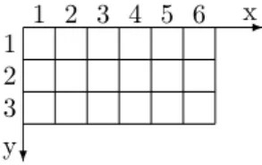
Figure 2.2: The system of coordinates used in our picture descriptions.
For m, n ∈ N, Σm,n is the subset of Σ∗∗ containing exactly all pictures of
sizem×n.
Σm,n={P|P ∈Σ∗∗∧rows(P) =m∧cols(P) =n}
Aprojection is every functionπ: Σ→Γ, where Σ and Γ are alphabets. We extendπon pictures and languages. LetP be a picture of sizem×nover Σ,L
be a picture language over Σ. Then
π(P) = [π(P(i, j))]m,n
π(L) ={π(P)|P ∈L}
In our descriptions, we use the system of coordinates in a picture depicted in Figure 2.2. Speaking about the position of a specific field, we use words like up, down, right, left, first row, last row etc. with respect to this scheme.
2.2
Two-dimensional Turing Machines
The two-dimensional Turing machine is the most general two-dimensional au-tomaton. It is a straightforward generalization of the classical one-dimensional Turing machine – the tape consisting of a chain of fields storing symbols from a working alphabet is replaced by a two-dimensional array of fields, infinite in both directions. The additional movements of the head, up and down, are al-lowed, preserving the possibility to move right and left. We emphasize, in our text, we consider the single-tape model only. However, it is possible to define multi-tape variants as well. A formal definition follows.
Definition 2 Atwo-dimensional Turing machineis a tuple(Q,Σ,Γ, q0, δ, QF),
where
?
-x
y
1 2 3 4 5 6 1
2 3 4
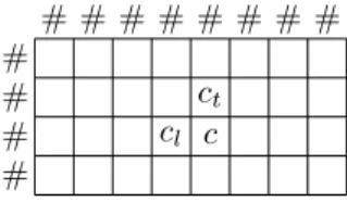
# # # # # # # # #
# # #
# # # # # # # # # # # #
Figure 2.3: Initial configuration – the figure on the left shows coordinates on the tape, where an input picture of size 4×6 is positioned. The figure on the right is the input bordered by #’s, which fill the remaining fields of the tape. The head scans the highlighted field (the top-left corner).
• Σ⊂Γ is an input alphabet
• Γ is a working alphabet
• q0∈Qis the initial state
• QF ⊆Qis a set of final states
• δ: Σ×Q→2Σ×Q×M is a transition function – M={L, R, U, D, N}
de-notes the set of the head movements (left, right, up, down, no movement) We assume there is always a distinguished symbol#∈Γ\Σcalled the background symbol.
Comparing to the formal definition of the one-dimensional Turing machine, there is only one difference – the set of the head movements contains two addi-tional elements.
LetT = (Q,Σ,Γ, q0, δ, QF) be a two-dimensional Turing machine,P ∈Σ∗∗ be an input picture.
Aconfiguration ofT is each triple (q,(xh, yh), τ), where
• q∈Qis the current state
• (xh, yh) is the coordinate of the head’s position
• τ is a mappingZ×Z→Γ assigning a symbol to each field of the tape (the field at coordinate (x, y) storesτ(x, y)). It is required that the subset of all fields storing a symbol different to # is always finite.
The computation of T is defined in the natural way, analogously to computations of Turing machines from the one-dimensional theory. Figure 2.3 shows the initial configuration of T. The head scans the field of coordinate (1,1). This field stores the top-left corner of the input (assuming P 6= Λ). During a computation, ifT is in a stateqand scans a symbol a, the set of all possible transitions is determined byδ(a, q). If (a0, q0, m)∈δ(a, q), thenT can
rewriteabya0, enter the stateq0 and move the head in the direction given by
m. A computational branch ofT halts whenever the control unit reaches some state in QF or whenever there is no instruction in δ applicable on the cur-rent configuration. The input is accepted if and only ifT can reach a state inQF.
T isdeterministic iff|δ(a, q)| ≤1 for each paira∈Γ, q ∈Qmeaning that at most one instruction can be applied at any given computational step.
T is #-preserving iff it does not rewrite any # by another symbol and does not rewrite any symbol different to # by #.
T isbounded iff it behaves as follows: WheneverT encounters #, it moves the head back in the next step and does not rewrite the symbol. When the input is Λ,T is bounded iff it does not move the head and rewrite at all.
T isfinite iff it does not rewrite any symbol.
For an input P, assuming each computational branch of T halts on P, let
t(P) be the maximal number of steps T has done among all branches (time complexity forP).
Definition 3 LetT = (Q,Σ,Γ, q0, δ, QF)be a two-dimensional Turing machine
andt(P)be defined for allP ∈Σ∗∗. Then,T is of time complexity
t1(m, n) = max
P∈Σm,nt(P)
In the literature, time complexity of a non-deterministic Turing machine is sometimes defined even in cases when the machine accepts, but there are also non-halting branches. However, for our purposes, the definition we have presented is sufficient, we will not work with such computations.
LetT be of time complexityt1:N×N→N. When we are not interested in
the dependency of time on picture size, we also define time complexityt2:N→
Nsimply as follows
t2(k) = max
m·n=kt1(m, n)
In this case, time complexity depends on the number of input fields only.
2.3
Notes on Computational Techniques
In this section we present two computational techniques and terms related to them. They will allow us to simplify descriptions of algorithms for Turing machines that we will design. The first term is the marker, the second term is theblock.
Working with markers is a commonly used technique. By a marker we mean a special symbol marking a field during some parts of a computation. To be more precise, let T = (Q,Σ,Γ, q0, δ, QF) be a Turing machine. T can be extended to have possibility to mark any field of the tape by the markerM in the following way: The working alphabet Γ is replaced by Σ∪(Γ× {0,1}) (we assume Σ∩(Γ× {0,1}) = ∅). Now, if a field stores (a, b), where a ∈ Γ and
b ∈ {0,1}, then b of value 1 indicates the presence of M in the field. A field storing a symbol from the input alphabet Σ is considered not to be marked. It is possible to extendT to support any constant number of different, mutually independent markers, let us sayM1, . . . , Mk. The working alphabet needs to be
extended to Σ∪Γ× {0,1}k in this case.
It is quite often suitable to organize the content of a working tape into blocks that are rectangular areas of tape fields. Formally, letT = (Q,Σ,Γ, q0, δ, QF)
b b b b b
l, b b, r
t t t t t
l, t t, r
l r
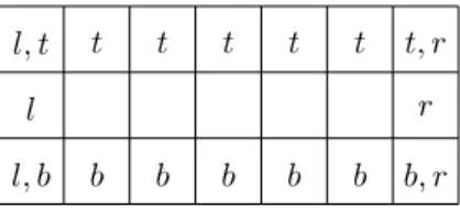
Figure 2.4: A block represented using markers t, l, b andr that are placed in the top, left, bottom, resp. right part of the perimeter.
be a two-dimensional Turing machine and letfx,y denote the tape field at co-ordinate (x, y). Then, for any tuple of integers (c1, c2, s1, s2), wheres1, s2>0,
the set
B={fx,y|c1≤x < c1+s1 ∧ c2≤y < c2+s2}
is a block. We say,B isgiven by (c1, c2, s1, s2).
Note that (c1, c2) is the coordinate of the top-left corner of B,s1, resp. s2
the number of columns, resp. rows. We can treat blocks like pictures and write rows(B) = s2, cols(B) = s1. We can also assign a content to a block, but,
comparing to pictures, this assignment is a function ofT’s configuration. For
i= 1, . . . s1; j = 1, . . . , s2, let B(i, j) be the field in B of coordinate (c1+i−
1, c2+j−1) (i.e. (i, j) is a relative coordinate within the block). Furthermore,
letsT(f, c) be the symbol of Γ stored in the fieldf in the configurationc. Then, the picture assigned toB inc isP, where P(i, j) =sT(Bi,j, c).
Theperimeter (orborder), denoted here byB0, ofBis the subset of its fields
given as follows:
B0 ={B(i, j)|i= 1∨j= 1∨i= cols(B)∨j= rows(B)}
When working with blocks during a computation, it is usually useful and sufficient to represent a block by markers placed in the border fields (i.e. fields ofB0) as it is shown in Figure 2.4.
LetB1, B2 be two blocks,B1 given by (x1, y1, s, t), B2 by (x1+d, y1, s, t),
whered≥t. It meansB2 is located right toB1and both blocks have the same
number of rows and columns. Let us assume the borders of both blocks are marked. By these circumstances, let us solve the task how to copy the content ofB1 intoB2.
An appropriate Turing machineT can work as follows: It starts having the head placed on the top-left field ofB1(we assumeT is able to locate this field).
The block is copied row by row, each row field by field. Two markers are used to mark the current source and destination. T records the scanned symbolain states, marks the scanned fieldf as ’read’, moves rightwards until it encounters the top-left field of B2 (it can be found thanks to border markers), writes a
to the detected field, marks the field as ’written’, moves back (leftwards) tof, clears the ’read’ marker, moves to the right neighbor off (which is the second field in the scanned row ofB1), marks it ’read’, stores the correspondent symbol
in states again, moves rightwards until the field marked ’written’ is detected, clears the marker, moves right by one field, copies the symbol recorded in states, places the marker ’written’, returns back to the field marked ’read’ and so on. WhenT reaches the end of the first row of B1 (at the moment the last field of
the row has been copied), it goes to the last field of the second row and starts to copy fields of this row in the reversed order (from right to left). In addition, it does not mark by ’written’ the field copied as the last one in the currently processed row ofB2, since this marker is not needed for the next iteration. The
procedure is repeated until all rows have been copied. The order in which fields are being copied is changed each timeT finishes a row.
As for the time complexity of the algorithm, one iteration (to copy a field) requires 2d+ 3 computational steps – two steps to check if the current source field is the last one to be copied in the current row,d−1 movements right to detect the field marked ’written’, one movement from this field to go to the proper destination field, dmovements back to the source field and one movent to the source field of the next iteration. When the algorithm ends, the head is placed on the bottom-right corner of B1 (T need not to move the head to the
next source field, when it returns back fromB2toB1and the bottom-right field
is the source field). Summing steps over all iterations, we see that the number of steps of the algorithm is not greater thans·t·(2d+ 3).
B1can be copied intoB2also ifB2is given by (x1+d, y1, s, t). The procedure
is analogous, time complexity remains the same. Even a general case, whenB2
is given by (x2, y2, s, t), can be handled similarly. ForT, it is only necessary to
be able to locate thei-th row ofB2when scanning thei-th row ofB1and vice
versa. It can be achieved by placing suitable markers before the procedure is launched. Moreover, if B1 andB2 overlap, the working alphabet is required to
code content of two block’s fields. Nevertheless, assuming the number of fields of the blocks is fixed, time complexity of the procedure is linear in the distance (measured in fields) between the top-left corners ofB1andB2- the distance is
|x1−x2|+|y1−y2|.
We will refer to the described technique using the termcopying a block field by field.
Chapter 3
Two-dimensional
Finite-state Automata
3.1
Finite-state Automaton
Definition 4 A two-dimensional finite-state automaton is every tuple
(Q,Σ, q0, δ, QF), where (Q,Σ,Σ∪ {#}, q0, δ, QF) is a two-dimensional finite
bounded Turing machine.
As we have already mentioned in section 1.1, we abbreviate a two-dimensional finite-state automaton byF SA, a deterministicF SAbyDF SA(we follow the notation in [20]). We use these abbreviations prior to one-dimensional finite-state automata. If we need to refer them, we will emphasize it explicitly. Since aF SAdoes not perform any rewriting, its working alphabet consists of elements in the input alphabet and the background symbol, thus it is fully given by a tuple of the form (Q,Σ, q0, δ, QF).
Finite-state automata have been studied by many authors. F SA’s working over pictures consisting of one row behave like two-way one-dimensional state automata that are of the same power as one-way one-dimensional finite-state automata. It means, F SA’s can be considered as a generalization of one-dimensional finite-state automata. The question that arises is what are the properties of the class L(F SA). Is this class a good candidate for the base class of the theory of two-dimensional languages, analogously to the class of regular languages? We list some of the most important properties of L(F SA) andF SA’s (as they are given in [20]).
• L(F SA) is not closed under concatenation (neither row or column)
• L(F SA) in not closed under complement
• L(DF SA)6=L(F SA)
• The emptiness problem is not decidable forF SA’s.
Example 2 To demonstrate capabilities ofF SA’s, let us define the following language over Σ ={a, b}.
L={AdB|A∈ {a}∗∗∧B ∈ {b}∗∗∧rows(A) = cols(A) = rows(B) = cols(B)}
L contains exactly each picture of sizen×2n(n∈N) consisting of two parts - the left part is a square ofa’s, while the right part a square ofb’s. We show thatLis inL(DF SA). LetP be an input,Abe aDF SAwe construct. It can easily perform these verifications:
• Checks if all rows are of the form aibj for some global constantsi, j. To do it,Ascans row by row, in a row, it verifies if there is a sequence ofa’s followed by a sequence of b’s and, starting by the second row, whenever it detects the end of the sequence of a’s, it checks if the correspondent sequence of a’s in the row above ends at the same position - this can be tested locally.
• Moves the head to the top-left corner, then, moves it diagonally (one field right and one field down repeatedly) until the last row is reached. In the field reached in the last row, Achecks whether it containsa.
• Moves the head right by one field, checks if the field contains b, moves diagonally right and up until the first row is reached. Finally, Achecks if the movement has ended in the top-right corner ofP.
3.2
Finite-state Automata over One-symbol
Al-phabet
In this section we will study F SA’s working over one-symbol alphabets. We prove a theorem allowing to show that some specific picture languages over one-symbol alphabet cannot be recognized by aF SA. As a consequence, we prove that L(F SA) is not closed under projection. As the properties we have listed in the previous section, this result is also different comparing to the class of regular languages.
For a one-symbol alphabet Σ (where|Σ|= 1), we use [m, n]Σto denote the
only picture over Σ of size m×n. When it is clear from the context which alphabet Σ is referred, we simply write [m, n].
We can prove a kind of pumping lemma for picture languages fromL(F SA) over one-symbol alphabets.
Proposition 1 Let Abe aF SA working over a one-symbol alphabetΣ. LetA have kstates. If A accepts a pictureP such that m= rows(P), n= cols(P)≥
1 +k·m, then, for alli∈N,A accepts[m, n+i·(m·k)!]too.
Proof. LetC={Ci}ti=0be an accepting computational branch ofA. A
configu-ration ofA is fully determined by the head position, the current state and size
m×n. Sincem,nare fixed during the whole computation, we consider elements ofCto be triples (i, j, q), wherei∈ {0, . . . , m+ 1}, resp. j∈ {0, . . . , n+ 1}is a horizontal, resp. vertical position of the head andq∈Q. Note thatAcan move the head one symbol out of the area of P, thus i, resp. j can be 0 or m+ 1, resp. n+ 1.
LetC0= (r0, n, q0) be the configuration inC in which the head ofAreaches
the last column of P first time. (If the head never reaches the last column it is evident thatA accepts every picture [m, n+l] for any integerl, so the proof can be easily finished here in this case.) Next, let C1 be the only contiguous
subsequence ofC satisfying
• the first element is a configuration, in which the head scans a field of the first column ofP
• no other element inC1(except the first one) is a configuration, where the
head scans a field of the first column
• the last element ofC1 isC0
Finally, we define C2 to be a subsequence of C1 (not necessary contiguous) of
lengthm·k+1, where eachi-th element (i= 1, . . . , m·k+1) is the configuration among elements ofC1, in which the head ofAreaches thei-th column first time.
Since|C2|=k·m+1, there are at least two configurations inC2such that the head
is placed in the same row andAis in the same state. Let these configurations be Ct1 = (r, c1, q) and Ct2 = (r, c2, q), where t1 < t2 and thus c1 < c2. We
emphasizeC2⊆ C1guaranteers that, during the part of the computation starting
by thet1-th step and ending by thet2-th step, the head ofAcan never scan the
symbol # located in the column left toP. Let Ct3 =C
0 and p=c
2−c1. Now, let us consider what happens if P is
extended toP0= [m, n+p] andAcomputes onP0. There exists a computational
branch that reaches the last column of P0 first time after t
3+t2−t1 steps
entering the configuration (r0, n+p, q0). Acan compute as follows. It performs
exactly the same steps that are determined by the sequence C0, C1, . . . , Ct2.
After that it repeats steps done during theCt1, . . . , Ct2 part, so it ends after t2−t1additional steps in the configuration (r, c2+p, q). Next, it continues with
Ct2, . . . , Ct3, reaching finally the desired configuration.
Instead of P0, it is possible to consider any extension of P of the form
[m, n+b·p] for any positive integer b. A can reach the last column in the stateq0 having its head placed in ther0-th row again. It requires to repeat the
Ct1, . . . , Ct2 partbtimes exactly.
Furthermore, we can apply the given observation on next computational steps ofA repeatedly. For A computing over P, we can find an analogy to C2
for steps following after the t3-th step. This time A starts scanning the last
column of P and the destination is the first column. We can conclude again that, for some periodp0,Acan reach the first column in the same row and state
for all pictures of the form [m, n+b·p0], b ∈ N. Then, there follows a part,
whenAstarts in the first column and ends in the last column again, etc. Since a period is always less thanm·k+ 1, (m·k)! is surely divisible by all periods. Hence, if a picture [m, n+i·(m·k)!] is chosen as an extension ofP, then, there is a computation ofAfulfilling: wheneverAreaches the first or the last column, it is always in the same state and scans the same row in both cases (meaningP
and the extended picture). Finally, during some movement of the head between the border columns ofP, ifA accepts before it reaches the other end, then it
accepts the extended picture as well. ut
Note that it is possible to swap words ”row” and ”column” in the lemma and make the proof analogously for picturesP fulfilling rows(P)≥1 +k·cols(P).
We have found later that Proposition 1 has been already proved ([11]), thus this result is not original.
A stronger variant of Proposition 1 can be proved for two-dimensional de-terministic finite-state automata.
Proposition 2 Let A be a DF SAworking over a one-symbol alphabetΣ. Let Ahavekstates. IfAaccepts a pictureP such thatm= rows(P),n= cols(P)≥
1 +k·m, then, there is an integer s, 0 < s≤ k!·(mk)2k such that, for any
i∈N,[m, n+i·s] is accepted byAtoo.
Proof. The main idea of the proof remains the same as it was presented in the proof of Proposition 1. The only different part is the estimate of the number of all possible periods. We show that in the case of DF SAwe can encounter at most 3kdifferent periods. Moreover,kof these possible periods are less then or equal tok(the remaining periods are bounded bym·k again).
Let us consider a part of the computation of A that starts and ends in the same row and state, that never reaches left or right border column of #’s and that is the minimal possible with respect to the period, i.e. it cannot be shortened to a consecutive subsequence to obtain a shorter period. Let the steps of the considered part of the computation be given by a sequence of configurationsC={Ci}it2=t1, whereCi= (ri, ci, qi). We havert1=rt2,qt1 =qt2.
We investigate two situations:
1) The head ofAdoes not reach the first or last row ofP during C
2) The head ofAreaches the first or last row ofP
Ad 1). We show that the period cannot be longer thank. By contradiction, let
t2−t1> k. Then, there is a pair Ci, Cj ∈ C, i < j < t2, such that the states
ofArelated to these configurations are not the same (qi6=qj). Now, ifri=rj, it contradicts to the minimality of the period of C. Otherwise, if ri 6= rj, let us say ri < rj (the second case is similar), then after performing j−i steps, the vertical coordinate of the head’s position is increased by rj−ri and A is again in the same state. It means, the vertical coordinate is being incremented in cycles of lengthj−itill the bottom ofP is reached, which is a contradiction. Ad 2). Since A is deterministic, the length of the period, i.e. t2−t1, is
uniquely determined by the stateAis in when it reaches the top, resp. bottom row ofP. It means there are at most 2ksuch periods.
All periods of the first type divide k!. Each period of the second type is bounded by m·k, thus all these periods divide a positive integer b less than (mk)2k. It means, for each i∈N, [m, n+i·k!·b] is accepted byA.
u t
Definition 5 Let Σbe a one-symbol alphabet,f :N+→N+ be a function. We
say that a languageL overΣ representsf if and only if 1. ∀m, n∈N+[m, n]
Σ∈L⇔n=f(m)
b b b b b b b b b b b b b b a a a a a a a a b b a a b
Figure 3.1: PictureP3.
For a fixed Σ such that|Σ|= 1, we denote the language representing f by
Lf, i.e.
Lf={[n, f(n)]Σ|n∈N+}
We also sayf is represented byLf.
Theorem 1 Let f :N+→N+ be a function such thatf =o(lin). Then,L
f is
not in L(F SA).
Proof. By contradiction. Let A be a F SA recognizing Lf and let k be the number of states ofA. Sincef =o(lin), there is an integern0such thatf(n0)≥
(k+ 1)·n0≥k·n0+ 1. By Proposition 1, it holds [n0, f(n0) + (k·n0)!]∈Lf.
It is a contradiction. ut
Example 3 Let L be a language consisting exactly of all pictures over Σ =
{a} having the number of columns equal to the square of the number of rows. Formally,L={[n, n2]|n∈N+}. Theorem 1 impliesL /∈L(F SA).
We shall note again that the result given in Example 3 can be found in the literature ([6]).
Example 4 We define a recurrent sequence of pictures {Pi}∞i=1 over the
al-phabet Σ ={a, b}. 1. P1=b
2. For alln≥1,
Pn+1= (PndVndSn) dHn+1
whereSn the rectangle over{a}of sizen×2n,Vn is the column ofb’s of lengthnandHn+1 is the row ofb’s of length (n+ 1)2.
Note that for every picturePn it holds rows(Pn) =n, cols(Pn) =n2(this result can be easily obtained by induction onn). We defineL={Pn|n∈N+}. Figure 3.1 shows an example of a picture inL.
Lemma 1 The languageLin Example 4 can be recognized by aDF SA. Proof. We describe how to construct aDF SA ArecognizingL. The computa-tion is based on gradual reduccomputa-tions of an inputP to sub-pictures. IfP =Pn+1
for some positive integern, then the sequence of sub-pictures produced by the process is Pn, Pn−1, . . . , P1. Moreover, the produced sequence is always finite
andP1 is its last element if and only ifP ∈L.
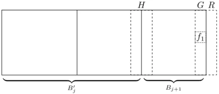
Let us take a closer look at the procedure performing one reduction. We consider the content of the tape to be as it is shown in Figure 3.2. The input
H
P0 V S
D G
C E F
# .. .
b· · · · · ·b
.. .
· · · #
b
.. . # · · ·
.. .
Figure 3.2: Division ofP into sub-pictures. IfP should be inL,S is required to be a rectangle of sizek×2k,V a column ofb’s andH a row ofb’s. P0 is the
product of the procedure. C,D,E,F andGare important fields ofP referred in our description.
to the procedure is the pictureP. The head scans the bottom-right corner ofP
(denoted byC). P is bounded by the background symbol # on the left and top side, the right and bottom borders are formed ofb’s. The goal of the procedure is to divideP into sub-pictures P0,S,V andH.
Acomputes as follows (note that Ahalts immediately and rejects the input if it founds that one of the listed conditions is not satisfied). First of all, A
moves the head left until the end of H is reached. During this movement, it verifies if all symbols ofH areb’s. Moreover, it checks if the row aboveH is of the form biaj, i, j ≥ 1. (It means A does not perform pure movement to the left – it goes up and down, before it moves left by one field.) The last row of
P0 must contain b’s only, otherwise P0 cannot be equal to some Pi. When A
finishes the verification, it is able to find the field D, since it is the leftmost field of H having the top-right neighboring field that contains a. A continues by moving the head to D and then goes trough all fields of V to ensure all of them contain b. After that, A moves its head to the top-right neighbor of D
and starts to verify if all fields of S contain a. It is done column by column.
A moves up until # is scanned. Then, the head is moved vertically back to
H followed by one movement to the right. A continues by checking the second column, etc. Now, to complete the verification ofS requires to check whether it is a rectangle of sizek×2k(k∈N+). Aplaces the head overE, then, moves
it diagonally toF (it performs three movements repeatedly – left, left and up). Reaching the border exactly inF indicates thatS is of the required size.
Finally, A moves the head to G. At this moment, the whole procedure is finished andAis ready to perform it again (on P0).
Before the process of reductions can be launched,Amust move the head to the bottom-right corner of the input. The process ends ifAdetects that some picture P cannot be divided correctly into sub-pictures as it was described in the previous paragraphs, or ifP1 is the result of some reduction. Acan detect
P1 when the head is placed over the field G. If G is the top-left corner of the
input and it contains b, then P1 has been obtained. One more remark – note
that when A performs the first reduction and the whole input to A is taken as an input to the procedure, then it is bounded by #’s only, there are nob’s. However, it should be obvious that this case can be distinguished and handled
easily. ut
It is a known fact that the class of one-dimensional regular languages is closed under homomorphism and since a projection is a special case of homomorphism, the class is closed under projection as well. We can show that the classes
L(F SA),L(DF SA) do not share this property.
Theorem 2 The classesL(F SA),L(DF SA)are not closed under projection. Proof. LetL1 be the language in Example 3 andL2 the language in Example
4. Let us define a projectionf : {a, b} → {a} such thatf(a) =f(b) =a. We shall see thatf(L2) =L1. SinceL2can be recognized by a deterministic
finite-state automaton andL1cannot be recognized by a non-deterministic finite-state
automaton, the theorem is proved. ut
3.3
Simulation of Finite-state Automata by
De-terministic Turing Machines
In this section we study how for a given two-dimensional non-deterministic finite-state automaton to construct a two-dimensional deterministic bounded Turing machine recognizing the same language. Our goal is to obtain machines optimized with respect to time complexity.
Questions regarding a relation ofF SA’s to determinism were also studied by P. Jiricka and J. Kral in [10], where the simulation ofF SA’s by two-dimensional deterministic forgetting automata is presented. However, in this case, the aim was to show the existence of such a simulation rather than to deal with time complexity.
We start with a relatively simple and straightforward simulation ofF SA’s. Proposition 3 Let A be a F SA recognizing L in time t(m, n). There is a bounded deterministicT M T such thatT recognizesLin timeO(t(m, n)·m·n). Proof. We will construct aDT M T. LetA= (Q,Σ, q0, δ, QA) and letP be an
input picture of sizem×n. We can assumeP is non-empty, sinceT can decide immediately if the empty picture should be accepted or not.
During the computation,T records a subset ofQin each field of the portion of the tape containing P. For a field, the subset represents states in whichA
can reach the field. At the beginning, all fields store empty subsets except the top-left corner which stores {q0}. Subsets are updated in cycles. During one
cycle, T goes through all fields of P, e.g. row by row. When scanning a field
f, it reads the subset currently recorded in f (let it beQf) and considers all transitions thatAcan perform in one step when it is in a state inQf having its head placed overf. By these all possible steps,T updates Qf and the subsets recorded in neighbors off to which the head can be moved (in another words,
T adds new states detected to be reachable).
Whenever T encounters that a state in QA is reachable in some field,P is accepted. During a cycle,T memorizes in its state, whether it has updated at least one subset. If no update has been done, it indicates that all reachable
# Mi i
z }| {
Ai
i
z }| {
Mi+1
i
z }| {
Ai+1 #
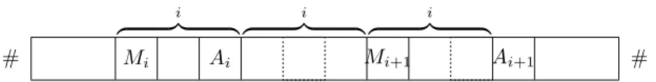
Figure 3.3: A portion of the tape containing markersAi,Mi,Ai+1,Mi+1. The
distance betweenAi andAi+1is 2·i+ 1.
pairs of state and position have been already detected, thusT halts and rejects
P.
It requires time O(m·n) to complete one cycle. We can see that if A can reach some field f in state q in time t1, then T detects the pair (f, q) to be
reachable by thet1-th cycle has been finished. It impliest(m, n) + 1 cycles are
required to calculate subsets of reachable states maximally, thusP is correctly accepted or rejected in timeO(t(m, n)·m·n). ut
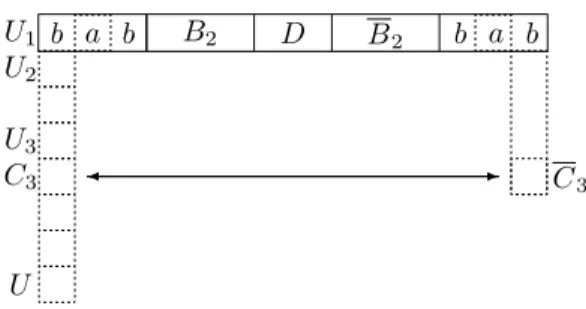
Lemma 2 It is possible to construct a one-dimensional deterministic bounded T M T that for any non-empty stringwover an alphabetΣcomputes the number k=bp|w|cand represents it by a marker placed in thek-th field ofw. Moreover, T works in time t(n) =O(n32).
Proof. Letwbe an input of lengthn >0. We constructT of the required type computingbnc.
LetS ={ai}∞i=1 be a sequence, whereai=i2 for eachi∈N+. The idea of the computation is to successively place markersA1, A2, . . . , Ak on fields ofw, eachAi to be in the distanceai from # precessing the leftmost field ofw. It is evident that ifk=b√nc, thenAk is the rightmost marker still positioned inw. Except markers Ai, T will also use auxiliary markers Mi. For eachAi, the marker Mi is placed in the distance ai−1 to the left from Ai. Note that all markersAiare represented using the same symbol,Aidenotes just an occurrence of the symbol on the tape (similarly forMi’s).
The computation starts by placing A1 andM1 on the first field ofw.
Posi-tions of next markers are determined inductively. Let us assumeAi andMi are correctly placed on the tape. Mi+1 should be in the distance
(i+ 1)2=i2+ 2·i+ 1 =a
i+ 2·i+ 1
It means, it is sufficient to copy the block starting byMiand ending byAiafter
Ai two times. Ai+1is putted after the second copy of the block,Mi+1is placed
on the first field of the second copy. All is illustrated in Figure 3.3.
IfT encounters the end ofw, it immediately stops placing markers and starts to count how many markers Ai there are on the tape. It means,T moves the head to the first field of w, removes A1 and initializes by 1 an unary counter,
which will represent the desired value in the end. Then, T repeatedly moves right until it detects some marker Ai, removes it, moves back and increments the unary counter. WhenT encounters the end ofw, allAi’s have been counted, soT halts.
It remains to estimate time complexity of the computation. AssumingT has placedAi,Miand the head is scanning the field containingAi, to place the next
pair of markers requires timec1·i2+c2, wherec1andc2are suitable constants.
The first copy of the block is created copying field by field in timec1·i2. The
second copy is created using the first copy, time is the same. Mi+1 is marked
after the the first copy is created,Ai+1 after the second copy is created. Both
require constant timec2. We derive
k+1
X
i=1
c1·i2+c2≤c1·
k+1
X
i=1
(k+ 1)2+c
2=c1·(k+ 1)3+c2·(k+ 1) =O
³
n32
´
WhenTcounts the number of markersAiduring the second phase, one marker is processed in time at mostn, thus the total time of this phase isO(n·k) =O(n32)
again. ut
Lemma 3 It is possible to construct a two-dimensional deterministic bounded T M T computing as follows. Let P be an input picture toT, next, let
m= min(cols(P),rows(P))
n= max(cols(P),rows(P))
k=b√nc
T checks whether k ≤m. If so, it represents k in unary in the first row, resp. column (depending on which of these two is of a greater length). Otherwise it halts. Moreover,T is of time complexityO¡min(m, k)3¢.
Proof. First of all,T compares values cols(P) and rows(P). It starts scanning the top-left corner. Then it moves the head diagonally, performing repeatedly one movement right followed by one movement down. Depending on during which of these two movements T reaches the background symbol first time, it makes the comparison.
Without loss of generality, letm= rows(P)≤cols(P) =n. T marks them -th field of -the first row. Again, -this field is detected moving -the head diagonally, starting in the bottom-left field. After thatT uses the procedure of Lemma 2 to compute k, but this time with a slight modification – whenever a field is marked by someAi, T increases the counter immediately (it does not wait till the end to count allAi’s – it should be clear that this modification does not have an impact on time complexity). If the counter exceeds m, T stops the computation.
To compare the number of rows and columns as well as to mark the distance
mrequires time O(m). If k≤m, thenT computeskin time O(n32) =O(k3),
otherwise it takes time O(m3) to exceed the counter. It implies T is of time
complexityO¡min(m, k)3¢. ut
Proposition 4 Let A= (Q,Σ, q0, δ, QA)be a FSA recognizing Lover Σ. It is
possible to construct a two-dimensional deterministic bounded Turing machineT that for each pictureP overΣof sizem×n, wheremin(m, n)≥ bmax(m, n)12c, decides whether P is inLin time t(m, n) =O(min(m, n)·max(m, n)32). Proof. LetA= (Q,Σ, q0, δ, QA) be aF SArecognizingL,P be an input picture
which of these numbers is greater (if any). It is again done by moving the head diagonally in the right-down direction, starting at the top-left field. Without loss of generality, let m ≤ n. By the assumption of the theorem, we have
m≥ bn12c.
Comparing to the construction presented in the proof of Proposition 3, we will use a different strategy now. We will work with blocks (parts ofP) storing a mapping. For a block B, the related mapping will provide the following information (B0 denotes the perimeter ofB).
• For each pair (f, q), wheref ∈B0 andq∈Q, the mapping says at which
fields and in which states A can leave B if it enters it at the field f, in the state q (to be more precise, when we speak about leaving the block, we mean, when Amoves the head outside B first time, after it has been moving it within the block).
• For each pair (f, q), the mapping also says if A can reach an accepting state without leaving B, by the assumption it has entered it at the field
f, in the stateq.
If the whole area ofP is divided into a group of disjunct blocks, it is sufficient to examine movements of the head across the blocks only to find out whether
Aaccepts P. We will need to solve what size of the blocks is optimal and how to compute the mappings.
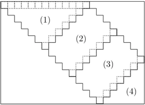
First of all, we will give details on how a mapping is stored inB. Let max(rows(B),cols(B))≤2·min(rows(B),cols(B))−1 (1)
For i = 1, . . . ,rows(B), resp. j = 1, . . . ,cols(B), let Ri, resp. Cj be the i-th row, resp. j-th column of B. Three functions, we are going to define now, form an equivalent to the mapping. They will also help to make the text more readable.
• S : B0×Q → 2B0×Q
, where S(f, q) is the set containing exactly each (f0, q0)∈B0×Qsuch thatAin qscanningf can reachf0 in the stateq0
without leaving the area of B.
• acc :B0×Q→ {true,false}, where acc(f, q) = true iffA inq scanningf
can reach some state in QAwithout leaving B.
• s:B0×Q×B0→2Q, where
s(f, q, h) ={q0|(h, q0)∈S(f, q)}
A mapping is fully determined bySand acc, since, ifT knows states reachable in a field ofB0, it can easily compute in which statesAcan leaveBfrom this field.
For each pairf ∈B0, q ∈Q, it could possibly hold that |S(f, q)| =|B0| · |Q|,
thus it is clear thatS(f, q) cannot be stored inf directly. A space linear in|B0|
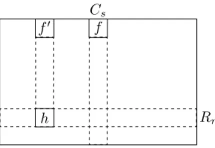
must be assigned to it. Figure 3.4 shows one possible solution of how to achieve it.
Let us assume f is thes-th field of the first row ofB as it shown in Figure 3.4. Moreover, let cols(B)≤2·rows(B)−1. Then,Csand Rr, where
r=
½
s ifs≤rows(B)
2·rows(B)−s otherwise store values ofS forf and eachq∈Qas follows: