Scalable Ensemble Information-Theoretic
Co-clustering for Massive Data
Qizhen Huang, Xiaojun Chen, Joshua Zhexue Huang, Shengzhong Feng, Jianping Fan
Abstract—Co-clustering is effective for simultaneously clus-tering rows and columns of a data matrix. Yet different co-clustering models usually produce very distinct results. In this paper, we propose a scalable algorithm to co-cluster massive, sparse and high dimensional data and combine individual clustering results to produce a better final result. Our algorithm is particularly suitable for distributed computing environment, which have been revealed in our experiments, and it is imple-mented on Hadoop platform with MapReduce programming framework in practice. Experimental results on several real and synthetic data sets demonstrated that the proposed algorithm achieved higher accuracy than other clustering algorithms and scale well.
Index Terms—ensemble learning, co-clustering, MapReduce
I. INTRODUCTION
Co-clustering, also called bi-clustering [1], [2], two-mode clustering [3], or two-way clustering [4], is a method of simultaneously clustering rows and columns of a data matrix. Recently, it has been widely used in numerous practical applications, including simultaneously clustering documents and words in text mining [5], [6], genes and experimental conditions in bioinformatics [2], [7], users and movies in recommender systems [8]. However, current co-clustering technologies face two main problems when handling massive data, such as data with millions of records and thousands of features. On the one hand, it is impossible to find an appropriate initial partition from large data so as to achieve a good clustering result. On the other hand, it is difficult, if not impossible, to cluster such massive data with serial algorithms running on single machines.
There exist three types of methods mainly in co-clustering. Code length method uses the MDL principe to automatically select the number of row and column clusters [9]. However, it only handles binary matrix. Mean squared distance-based co-clustering algorithm is an efficient node-deletion algorithm which is proposed to find submatrices that have low mean squared residue scores in gene expression data [2], but it only produces one cluster at a time. Information-theoretic co-clustering(ITCC) is able to findκ×`(κ,`are the number of row and column clusters, respectively) co-clusters simultane-ously [5]. It can avoid dimension curse problem [10] since there is no need to compute distances between two objects but only mutual information.
Manuscript received January 12, 2012; revised January 21, 2012. This work is supported by Shenzhen Key Laboratory of High Performance Data Mining (grant no. CXB201005250021A).
X. Chen (corresponding author) is with Shenzhen Institutes of Advanced Technology, Chinese Academy of Sciences, 1068 Xueyuan Avenue, Shen-zhen University Town, ShenShen-zhen, P.R.China (phone: (86)-755-863- 92346; fax: (86)-755-863-92346; e-mail: [email protected]).
Q. Huang, J. Huang, S. Feng and J. Fan are with Shenzhen Institutes of Advanced Technology, Chinese Academy of Sciences, 1068 Xueyuan Av-enue, Shenzhen University Town, Shenzhen, P.R.China (e-mail:{qz.huang, zx.huang, sz.feng, jp.fan}@siat.ac.cn).
Recent researches focused on distributed co-clustering for massive data. Papadimitriou et al. [11] designed a frame-work for a holistic approach focusing on code length-based co-clustering algorithm. Zhou et al. [12] implemented the sum squared distance-based co-clustering in a MPI environment. A parallel information-theoretic co-clustering algorithm using a cloud middle ware, FREERIDE, is pro-posed in [13]. However, there exits redundant computations, and FREERIDE is not an open platform. MapReduce is a simple programming model for distributed computing [14], [15], [16]. It abstracts away many low-level details such as task scheduling and data management, and conceptualizes a computational process as a sequence of Map and Reduce functions. If the data file is large, more data blocks are created and distributed on more computing nodes. The map and reduce functions are automatically dispatched to more computing nodes. Therefore, MapReduce model is scalable to large data.
In this paper, we present a scalable ensemble information-theoretic co-clustering(SEITCC) algorithm for massive data. We first build multiple different co-clusterings using ITCC algorithm, and then combine them to produce a final co-clustering with the evidence accumulating mechanism [17]. The reason for using ensemble clustering method is that it can improve the quality and robustness of clustering results [18]. To deal with massive data, our algorithm is designed particularly suitable for distributed computing envi-ronment. Massive data can be distributed into separate nodes, and our algorithm can generate multiple co-clusterings on different nodes in parallel. In practice, we implement our algorithm using MapReduce programming framework [19]. Multiple co-clusterings are generated with a pipeline of map and reduce operations. We have conducted experiments on clusters with 30 nodes installed with Hadoop. The re-sults have shown that our algorithm outperformed original ITCC algorithm in clustering accuracy and MapReduce’s distributed computing ability endows our model good scala-bility.
The remainder of the paper is organized as follows. Section 2 gives a brief introduction to information-theoretic co-clustering and the notion of cluster ensembles. Section 3 describes the proposed algorithm in details. In Section 4, we show the implementation details of our algorithm using MapReduce. Experimental results on both synthetic data and real data are presented in Section 5. Finally, we draw conclusions in Section 6.
II. PRELIMINARY
A. Information-Theoretic Co-clustering
distribution between two discrete random variables that take values over the rows and columns. A pair of maps from rows to row-clusters and from columns to column-clusters is defined as a co-clustering, and the optimal co-clustering is the one that leads to the largest mutual information between the clustered random variables. LetXandY be discrete random variables that take values in the sets{x1, . . . , xm}(rows) and
{y1, . . . , yn}(columns) respectively. Letp(X, Y)denotes the
joint probability distribution between X andY. The output of ITCC with κrow clusters and ` column clusters is two mapsCX andCY defined as:
CX:{x1, . . . , xm} → {xˆ1, . . . ,xˆκ}
CY :{y1, . . . , yn} → {yˆ1, . . . ,yˆ`}
The ITCC algorithm to minimize the loss in mutual information upon co-clustering is shown as follows:
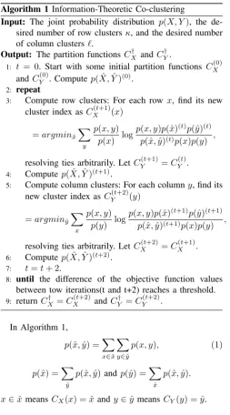
Algorithm 1 Information-Theoretic Co-clustering
Input: The joint probability distribution p(X, Y), the de-sired number of row clustersκ, and the desired number of column clusters`.
Output: The partition functionsCX† andCY†.
1: t = 0. Start with some initial partition functions CX(0) andCY(0). Computep( ˆX,Yˆ)(0).
2: repeat
3: Compute row clusters: For each rowx, find its new cluster index asCX(t+1)(x)
=argminxˆ X
y
p(x, y)
p(x) log
p(x, y)p(ˆx)(t)p(ˆy)(t) p(ˆx,yˆ)(t)p(x)p(y) , resolving ties arbitrarily. LetCY(t+1)=CY(t). 4: Computep( ˆX,Yˆ)(t+1).
5: Compute column clusters: For each columny, find its new cluster index asCY(t+2)(y)
=argminyˆ X
x
p(x, y)
p(y) log
p(x, y)p(ˆx)(t+1)p(ˆy)(t+1)
p(ˆx,yˆ)(t+1)p(x)p(y) , resolving ties arbitrarily. LetCX(t+2)=CX(t+1). 6: Computep( ˆX,Yˆ)(t+2).
7: t=t+ 2.
8: until the difference of the objective function values between tow iterations(t and t+2) reaches a threshold. 9: returnCX† =CX(t+2) andCY† =CY(t+2).
In Algorithm 1,
p(ˆx,yˆ) =X
x∈ˆx
X
y∈yˆ
p(x, y), (1)
p(ˆx) =X
ˆ
y
p(ˆx,yˆ)andp(ˆy) =X
ˆ
x
p(ˆx,yˆ).
x∈xˆ meansCX(x) = ˆxandy∈yˆmeans CY(y) = ˆy.
B. Clustering Ensemble
Let P represent the set of S partitions of data X (with
m objects), P={P1, . . . , PS}, where Ps={C1s, . . . , Ckss} is the s-th partition, Cls is the lth cluster in partition Ps,
which has ks clusters and nsl is the cardinality of C s l,
withPks
l=1n
s
l =m. The clustering ensemble problem is to
combine theS data partitions inPto find an “optimal” data partitionP∗.
The first step of clustering ensemble is to generate multiple different clustering partitions P. Commonly-used methods
includes: (a) employing different clustering algorithms; (b) using the same algorithm with different algorithmic parame-ter values or giving distinct initial partitions for each single clustering; (c) using different similarity measures between patterns.
The second step is to find an “optimal” data partition P∗. Strehl and Ghosh introduced some methods [18]. The first method is mutual information-based, but it is often computationally intractable, and tends to result in poor local optima. The other three methods are hypergraph-based. Data partitions in P are first transformed into a special type of
hypergraph and a specific hyper graph partitioning algorithm is used to partition the hypergraph to get the final clustering result. However, our experimental results have shown that these methods performed bad when the data set contains imbalanced clusters, which means that the number of objects in different clusters are greatly different. Recently, Fred et. al proposed an evidence accumulation method for combination of multiple clustering partitions. The key of this method is to compute am×mco-association matrixCfrom data partitions inP. The new matrix C can be viewed as a new similarity
matrix and then any clustering algorithm can be applied to find the final data partition.
III. SCALABLEENSEMBLEINFORMATION-THEORETIC CO-CLUSTERING
In this section, we present the main design of our algo-rithm SEITCC. Our cluster algoalgo-rithm generates multiple co-clusterings concurrently in a distributed system using ITCC with different initial partitions. Then we use the evidence accumulation ensemble learning method to produce the final cluster result.
A. Data Pre-processing
[image:2.595.46.300.263.720.2]Fig. 1. Data transformation procedure
B. Distributed Co-clustering
When dealing with massive data, one clustering is difficult to cluster the whole data set. It is beneficial to partition the integrated data into separate machines in a distributed system. One clustering can then do the clustering work over the subsets of the whole data set. In a distributed environment, the subsets of a data set are processed by one clustering in parallel in different machines. Specifically for ITCC, the key step is to updatep( ˆX,Yˆ)which is shown in Algorithm 1. Thus we should compute p( ˆX,Yˆ) for each subset in parallel. Let a probability distribution p(X, Y)
represent the input matrix of ITCC. Partition p(X, Y) by rows into R nodes in a distributed system. The data sets in different nodes are denoted as D = {D1, D2, . . . , DR}.
We further prove the following theorem, which makes sure the sum ofp( ˆX,Yˆ)computed in the distributed computing environment are equivalent to that computed in a single machine environment.
Theorem 1: The sum ofpi( ˆX,Yˆ)is equal top( ˆX,Yˆ), that
isPR
i=1pi( ˆX,Yˆ) =p( ˆX,Yˆ), where pi( ˆX,Yˆ)is computed
by the i-th machine in a distributed system, andy∈yˆis fixed when assigning rows to new clusters, similarly for column clustering if we transposep( ˆX,Yˆ)and fixx∈xˆ.
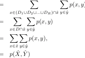
Proof:
Because pi( ˆX,Yˆ) = Px∈Di∩ˆx P
y∈yˆp(x, y) according to the data partition D ={D1, D2, . . . , DR} and equation (1)
in II-A, then p1( ˆX,Yˆ) +p2( ˆX,Yˆ) +. . .+pR( ˆX,Yˆ)
= X
x∈(D1∪D2∪...∪DR)∩xˆ X
y∈yˆ p(x, y)
= X
x∈D∩ˆx
X
y∈yˆ p(x, y)
= X
x∈ˆx
X
y∈yˆ p(x, y),
= p( ˆX,Yˆ)
We can then surely cluster data in a distributed environment using ITCC.
A cluster ensemble consists of multiple clusterings. Each clustering has its own clustering result over the same input data set. We obtain multiple cluster results at first. Unlike the one-way clustering algorithm, co-clustering needs to do row clustering and column clustering. We transpose the original probability distribution at first so that the column clustering job can be done with the transpose matrix using the same procedure as the row clustering job. The construction of multiple data partitions in a distributed system consists of the following key steps.
(1) In node i of a distributed system, assign each instance (row or column ofp(X, Y)) to a new cluster for each clustering. Thus, we can get the newCXs orCYs, where the cluster labelCXs(x) or CYs(y) is the new cluster index ofx-th row ory-th column in the sub data set i,
and a partial compressed matrixps
i( ˆX,Yˆ)for thes-th
clustering.
(2) For each clustering, sum up all the partial compressed matrices to prepare the new compressed matrix for the next iteration.
(3) Update the new membership functions CX or CY
and compressed matrix p( ˆX,Yˆ) for each clustering. Redistribute them to every node.
We summarize the construction of multiple co-clusterings in the pseudo code in Algorithm 2. After acquiring the multiple cluster results, we are able to combine them to produce an optimal result.
Algorithm 2Scalable Construction of Multiple Clusterings Input: The joint probability distribution p(X, Y), the de-sired number of row clusters κ, the desired number of column clusters ` , the number of nodes in a distribute systemR, and the number of the cluster modelsS. Output: The partition functions
CX1, CX2, . . . , CXS and CY1, CY2, . . . , CYS .
1: Transpose p(X, Y) to t(X, Y). Compute the marginal probabilities of every row and column. Obtainp(X)and p(Y).
2: Initialize randomly CX1, CX2, . . . , CXS and
C1
Y, C
2
Y, . . . , C S
Y . Compute the compressed matrices
p1( ˆX,Yˆ), p2( ˆX,Yˆ), . . . , pS( ˆX,Yˆ).
3: DistributeCX1, CX2, . . . , CXS andCY1, CY2, . . . , CYS , p1( ˆX,Yˆ), p2( ˆX,Yˆ), . . . , pS( ˆX,Yˆ), and p(X), p(Y)
into Rnodes;
4: Partitionp(X, Y)intoD={D1, D2, . . . , DR},t(X, Y)
into D0 ={D10, D20, . . . , DR0 }. 5: In each node i :
6: fors= 1 to S do
7: Compute row(column) clusters: For each row x or columny inp(X, Y), find its new cluster index as
CX(x) =argminxˆ X
y
p(x, y)
p(x) log
p(x, y)p(ˆx)p(ˆy)
p(ˆx,yˆ)p(x)p(y).
Lety ∈ yˆfixed. Or CY(y) =argminyˆ
X
x
p(x, y)
p(y) log
p(x, y)p(ˆx)p(ˆy)
p(ˆx,yˆ)p(x)p(y).
Let x ∈ xˆ fixed. And compute partial compressed matrixps
i( ˆX,Yˆ).
8: end for
9: fors= 1 to S do 10: Sum upps
i( ˆX,Yˆ). Obtainps( ˆX,Yˆ)
11: end for
12: Distribute the new partition functions and new com-pressed matrices to each node.
13: fors= 1 to S do
14: Compute the difference of the objective function val-uesobjs.
15: ifobjs is “small” (say10−3)then
16: Add the newCXs and newCYs into outputs. 17: else
18: Go to step 5 and repeat the subsequent operations. 19: end if
C. Ensembles
We use the evidence accumulation mechanism to combine the multiple co-clusterings. A cluster ensemble that has S clustering results overmobjects are denoted as follow:
P={P1, . . . , PS}.
Pis used to compute them×mco-association matrix. When
treating the co-occurrence frequency of the pattern pairs in the same cluster as votes for their association, the S cluster results of m patterns then can be mapped into a m×m co-association matrix:
C(i, j) = sij
S
where sij is the number of times the pattern pair (i, j) is
assigned to the same cluster among the S cluster results. Next, we use K-means implemented in a distribute manner to cluster the new matrix. K-means is a traditional clustering algorithm, which has been studied for almost a half century [21]. A distributed K-means was implemented in reference to Mahout K-means1in our experiments. When deciding which distance measure is suited for the similarity matrix, we did some experiments and find out that cosine distance measure performs better than other measurements over the data we used. For a big m, the distribute evidence accumulation method, using K-means method for achieving the final cluster result, is summarized in Algorithm 3.
Algorithm 3Ensemble Clustering using Evidence Accumu-lation with K-means
Input: m: number of objects,S: number of clusterings,P=
{P1, . . . , PS}: S data partitions.
Output: P∗: combined data partitions.
1: Initialization: Set the component values of a m-tuple vector v to zero. Set every entry of a m×m matrix C to zero.
2: foreachPs∈
P do
3: fori=0 tom−1 do 4: forj=0 tom−1 do 5: if P(i) =P(j)then 6: v(j)+ = S1
7: end if 8: end for 9: Recordvs
i. Reset the component values ofvto zero.
10: end for 11: end for
12: fori=0 tom−1 do 13: fors = 1 toS do 14: C(i)+ =vsi
15: end for 16: end for
17: Cluster the matrixCusing K-means. The clustering result is the final data partitionP∗.
IV. IMPLEMENTATION WITHMAPREDUCE
MapReduce is an advantageous distributed programming model, and it is suitable to implement the procedure of
[image:4.595.309.543.53.195.2]1 https://cwiki.apache.org/confluence/display/MAHOUT/K-Means+Clustering
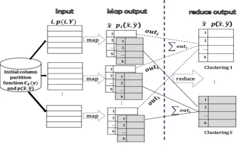
Fig. 2. MapReduce for construction of multiple clusterings
TABLE I REAL DATA SETS
DataSet number of
instances
number of features
class
20 news group 11268 5000 20
20 news group 5 2928 5000 5
20 news group 3 1762 5000 3
Amazon Reviews 1500 10000 50
Amazon Reviews 650 650 10000 50 Amazon Reviews 400 400 10000 50
libras 360 90 15
libras 10 270 90 15
libras 8 135 90 15
construction of multiple co-clusterings. We seek map and reduce functions to perform the alternating updates of row and column clusters in the Map-Reduce framework.
In map phase: The joint distribute probability p(X, Y)
and its transpose are stored on HDFS [14] as text files. The input key is the instance indexi, along with the vectorp(i, Y)
(or t(i, Y)) representing an instance as values. The initial column partition functions (or row partition functions for column clustering) andp( ˆX,Yˆ)are globally broadcasted to all mappers. Given this information, the mapper computes the locally optimal row labelCX(x)for each rowx(or column
labelCY(y)for each columny), as well as the compressed
matrices for S clustering models. We use model IDs as the intermediate keys. The intermediate values comprise of the partial objective function values, the partial compressed matrices and the membership information.
In reduce phase: The reducer sums up the partial com-pressed matrices from every mapper, computes the whole objective function values, and merges group members for each cluster label. The merging work for one clustering is arranged to one reducer. Figure 2 shows the procedure of map and reduce. In this figure, we illustrate only row clustering withκrow clusters andSclusterings. It is similar for clustering columns.
V. EXPERIMENTS
TABLE II SYNTHETIC DATA SETS
Data Set
number of instances
number of features
number of row clusters
number of col-umn clusters
D1 2,000,000 1,000 10 10
D2 1,000,000 1,200 5 4
D3 800,000 1,500 10 5
D4 500,000 2,000 10 10
A. Data Sets
Three real data sets which have the information of true labels are used to evaluate the accuracy of our method. 20 Newsgroups(NG20) is a collection of approximately 20,000 newsgroup documents, partitioned evenly across 20 different newsgroups which is from http://people.csail.mit.edu/jrennie/20Newsgroups/. Many of the newsgroups share similar topics and the boundaries between some groups are fuzzy. So we selected various subsets from this corpus in our experiments. The second and third data sets are downloaded from UCI repository. Amazon Commerce Reviews (“Reviews”) is used for authorship iden-tification in online writeprint which is a new research field of pattern recognition [22]. Its attributes include authors’ linguistic style such as usage of digit, punctuation, words and sentences’ length and usage frequency of words and so on. Libras is the official Brazilian sign language. It contains 15 classes of 24 instances each, where each class references to a hand movement type [23]. In each instance of Libras, every attribute has a non-zero value. But in “Reviews”, there are considerable zero values. Thus “Reviews” is extraordinary sparse. NG20 is less sparser than “Reviews”. We selected subsets from “Reviews” and Libras as NG20. The character-istics of these real data sets are described in Table I.
We have developed a data generator to generate data of various sizes. There is one instance per line, and each line contains feature values of the instance separated by blank space. Features are represented by feature order number and feature values. For example, the below data set contains 1 instance and 30 features. Features whose values are zero are not recorded.
5:0.029 9:0.005 16:0.017 23:0.004 26:0.038
Four data sets produced by this generator are shown in Table II.
B. Experiment Setup
30 machines were used in the experimental environment, each having eight 2.13GHz Intel(R) Xeon(R) processors and 25G memory, running CentOS Linux operating system. We used the latest stable version of Hadoop, hadoop-0.20.2, to form a MapReduce programming environment.
C. Accuracy
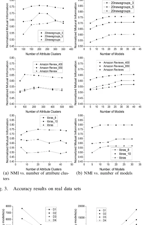
In this part, we evaluate the performance of our algorithm with accuracy. For the real data sets in Table I, we use normalized mutual information(NMI) [18] as the evaluation measure. To show how the instance clustering results change with the number of feature clusters, we tried different feature clusters for the three data sets in Table I. Figure 3(a) shows the NMI curve against the number of feature clusters where the number of clustering models is fixed. With the increment
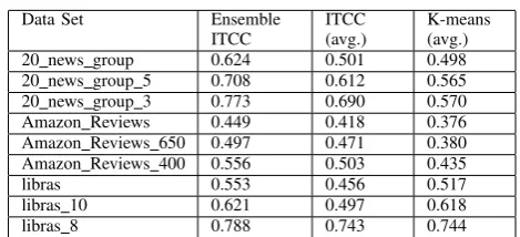
TABLE III ACCURACY COMPARISON
Data Set Ensemble
ITCC
ITCC (avg.)
K-means (avg.)
20 news group 0.624 0.501 0.498
20 news group 5 0.708 0.612 0.565 20 news group 3 0.773 0.690 0.570 Amazon Reviews 0.449 0.418 0.376 Amazon Reviews 650 0.497 0.471 0.380 Amazon Reviews 400 0.556 0.503 0.435
libras 0.553 0.456 0.517
libras 10 0.621 0.497 0.618
libras 8 0.788 0.743 0.744
[image:5.595.51.292.77.137.2]of numbers of feature clusters, the accuracy also increases, but the accuracy will decrease when the number exceeds a certain value range. Various subsets of the same data set reached their peak accuracy with different number of feature clusters. Figure 3(b) shows the NMI curve against the number of clustering models where the number of feature clusters is fixed. We notice that the accuracy increases with the increment of the number of models, but the accuracy only changes in a small range when the number of models exceeds a threshold. Finally, we find some critical points in different data sets where the accuracy nearly approaches to a limit value or a small range. Then, we did experiments on that point repeatedly and took the average of all the experiment results as our last accuracy of our algorithm. In Table III, we show the accuracy of our ensemble model, comparing with single ITCC and the Mahout K-means.
Table III shows that the accuracy of our algorithm gains a notable increase than the traditional cluster algorithm (K-means) when dealing with high dimensional and sparse data, but is similar to that of K-means for non-sparse data. It’s clear to see that the accuracy of ensemble ITCC is higher than single ITCC for all the data sets in our experiments. To sum up, our algorithm has good accuracy in dealing with high dimensional and sparse data.
D. Scalability
In this part, we have carried out two groups of experiments to evaluate the performance of scalability. In the first group of experiments, we fixed the number of clustering models as 20, then we constructed clustering ensembles for the data sets in Table II running on different numbers of nodes. We present the time of our algorithm in dealing with different sizes of data running on 10 nodes, 20 nodes and 30 nodes respectively in the left-chart of Figure 4. In the second group of experiments, we present the time curve of different numbers of models for different sizes of data running on 30 nodes in the right chart of Figure 4.
(a)NMI vs. number of attribute clus-ters
[image:6.595.55.289.56.421.2](b)NMI vs. number of models
Fig. 3. Accuracy results on real data sets
Fig. 4. Scalability results on large synthetic data sets
VI. CONCLUSIONS
In this paper, we have proposed a scalable ensemble information-theoretic co-clustering, which is focused on large scale data clustering problems. We constructed multiple clustering models to produce different data partitions parallel in a distributed environment. Finally, we took the ensemble result of multiple data partitions as the final clustering result. The experimental results demonstrated the superior performance of our algorithm against distributed K-means and individual information-theoretic co-clustering both on synthetic and real data sets.
In the future, we will further investigate the relationship between the ensemble result accuracy and the number of attribute clusters and the relationship between the ensemble result accuracy and the number of clustering models. Since the qualities of distinct clustering results are different, we will also investigate new methods to evaluate the weight of different clustering results and then use weighted information to combine them.
ACKNOWLEDGEMENTS
The authors would like to thank Baoxun Xu, Bingguo Li, Shuang Wang and Xianggang Zeng for their suggestions and feedback to this work.
REFERENCES
[1] J. Hartigan, “Direct clustering of a data matrix,” Journal of the American Statistical Association, pp. 123–129, 1972.
[2] Y. Cheng and G. Church, “Biclustering of expression data,” in Pro-ceedings of the eighth international conference on intelligent systems for molecular biology, vol. 8, 2000, pp. 93–103.
[3] I. Van Mechelen, H. Bock, and P. De Boeck, “Two-mode cluster-ing methods: astructuredoverview,” Statistical methods in medical research, vol. 13, no. 5, pp. 363–394, 2004.
[4] G. Getz, E. Levine, and E. Domany, “Coupled two-way clustering anal-ysis of gene microarray data,”Proceedings of the National Academy of Sciences, vol. 97, no. 22, p. 12079, 2000.
[5] I. Dhillon, S. Mallela, and D. Modha, “Information-theoretic co-clustering,” inProceedings of the ninth ACM SIGKDD international conference on Knowledge discovery and data mining. ACM, 2003, pp. 89–98.
[6] B. Gao, T. Liu, X. Zheng, Q. Cheng, and W. Ma, “Consistent bipartite graph co-partitioning for star-structured high-order heterogeneous data co-clustering,” inProceedings of the eleventh ACM SIGKDD interna-tional conference on Knowledge discovery in data mining. ACM, 2005, pp. 41–50.
[7] H. Cho, I. Dhillon, Y. Guan, and S. Sra, “Minimum sum-squared residue co-clustering of gene expression data,” inProceedings of the fourth SIAM international conference on data mining, vol. 114, 2004. [8] T. George and S. Merugu, “A scalable collaborative filtering framework based on co-clustering,” in Data Mining, Fifth IEEE International Conference on. IEEE, 2005, pp. 4–pp.
[9] D. Chakrabarti, S. Papadimitriou, D. Modha, and C. Faloutsos, “Fully automatic cross-associations,” inProceedings of the tenth ACM SIGKDD international conference on Knowledge discovery and data mining. ACM, 2004, pp. 79–88.
[10] K. Beyer, J. Goldstein, R. Ramakrishnan, and U. Shaft, “When is nearest neighbor meaningful?” Database TheoryłICDT99, pp. 217– 235, 1999.
[11] S. Papadimitriou and J. Sun, “Disco: Distributed co-clustering with map-reduce: A case study towards petabyte-scale end-to-end mining,” inData Mining, 2008. ICDM’08. Eighth IEEE International Confer-ence on. IEEE, 2008, pp. 512–521.
[12] J. Zhou and A. Khokhar, “Parrescue: Scalable parallel algorithm and implementation for biclustering over large distributed datasets,” in Distributed Computing Systems, 2006. ICDCS 2006. 26th IEEE International Conference on. IEEE, 2006, pp. 21–21.
[13] V. Ramanathan, W. Ma, V. Ravi, T. Liu, and G. Agrawal, “Parallelizing an information theoretic co-clustering algorithm using a cloud middle-ware,” inData Mining Workshops (ICDMW), 2010 IEEE International Conference on. IEEE, 2010, pp. 186–193.
[14] T. White,Hadoop: The definitive guide. Yahoo Press, 2010. [15] J. Venner,Pro Hadoop. Springer, 2009.
[16] C. Lam and J. Warren, “Hadoop in action,” 2010.
[17] A. Fred and A. Jain, “Combining multiple clusterings using evi-dence accumulation,”Pattern Analysis and Machine Intelligence, IEEE Transactions on, vol. 27, no. 6, pp. 835–850, 2005.
[18] A. Strehl and J. Ghosh, “Cluster ensembles—a knowledge reuse framework for combining multiple partitions,”The Journal of Machine Learning Research, vol. 3, pp. 583–617, 2003.
[19] J. Dean and S. Ghemawat, “Mapreduce: Simplified data processing on large clusters,”Communications of the ACM, vol. 51, no. 1, pp. 107–113, 2008.
[20] R. Fisher, “On the interpretation ofχ2 from contingency tables, and the calculation of p,”Journal of the Royal Statistical Society, vol. 85, no. 1, pp. 87–94, 1922.
[21] D. Steinley, “K-means clustering: A half-century synthesis,”British Journal of Mathematical and Statistical Psychology, vol. 59, no. 1, pp. 1–34, 2006.
[22] A. Frank and A. Asuncion, “UCI machine learning repository,” 2010. [Online]. Available: http://archive.ics.uci.edu/ml