Predicting Effect of Temperature Field on Sensitization of Alloy 690 Weldments

Predicting Effect of Temperature Field on Sensitization of Alloy 690 Weldments

Hwa Teng Lee

_{and Chun Te Chen}

Department of Mechanical Engineering, National Cheng Kung University, Tainan 701, Taiwan, R. O. China

The present study develops two 3-D finite element (FE) thermal models of the temperature field induced within an Alloy 690 butt weld fabricated using the two-pass GTA welding and the laser beam welding (LBW) methods, respectively. The welding thermal cycles of the two welding methods are simulated using ANSYS software based upon a moving heat source model and the high-temperature thermal physical property data are derived in the JMatPro database. The validity of the numerical model is confirmed by comparing the simulation results with the corresponding experimental findings. Agreement is found between the numerical results for the temperature field and the experimental temperature measurements. In addition, the FEM models we use can help us estimate the range and size of the sensitization zone and the time duration of the sensitization temperature. Overall, the results provide useful insight into the sensitization tendencies of Alloy 690 weldments. [doi:10.2320/matertrans.M2011147]

(Received May 18, 2011; Accepted June 29, 2011; Published August 25, 2011)

Keywords: finite element method, nickel based superalloys, welding, sensitization, heat-affected zone, transient temperature field

1. Introduction

Alloy 690, an austenitic, low-carbon, and high-chromium modification of Alloy 600, was developed to resist stress corrosion cracking and general corrosion in high temperature aqueous environments associated with nuclear steam gen-erators. In the late 1980s, it was reported that Alloy 600 is susceptible to pitting, stress corrosion cracking (SCC), and intergranular stress corrosion cracking (IGSCC) as a result of a sensitization effect during cooling in which Cr-rich carbides (e.g. Cr23C6and Cr7C3) are precipitated at the grain boundaries. As a result, serious doubts were raised as to its suitability for such critical applications as nuclear power plant components by Scott1)_{and Harrodet al.}2)_Researchers have generally resolved this safety issue through the use of alternative materials, as done by Kim and Moon,3) _{or the} application of more sophisticated welding techniques such as laser beam welding (LBW) or electron beam welding (EBW). Compared to the traditional GTAW welding process, Nd:YAG LBW is characterized by a more con-centrated heat input, a higher welding speed, and a faster cooling rate. As a result, the weldment has a narrower heat-affected zone (HAZ), a lower residual stress, and a reduced susceptibility to carbide precipitation during heating and cooling.4) _{In addition, Nd:YAG LBW has the advantage} that the heat energy can be supplied remotely to the welding area via an optical fiber, and thus Kim et al.5) _reported that Nd:YAG LBW is an ideal solution for the repair of components in hazardous environments such as nuclear reactor plants.

Welding is a highly complex physical phenomenon, influenced by many parameters including the heat trans-mission mode (i.e. conduction, radiation, and convection), the geometry and properties of the workpiece, the phase transformations caused by the heat input in the welding procedure, and the welding specifications, e.g. the voltage, current, choice of electrode, welding speed, and intensity of heat input. Analytical solutions and heat source style for

the temperature field induced during welding models were reported.6–10) _{However, analytical methods are limited in} their ability to clarify the physical phenomena which take place during a typical welding operation. Accordingly, recent studies have generally employed some form of numerical modeling approach to simulate the welding process. An excellent review of the thermal modeling of laser welding and related processes is provided by Mackwood.11)_Although various numerical modeling techniques are available, FEM tends to be the most widely used due to its convenience.12–14) Although computer simulations provide the means to obtain detailed insights into the basic phenomena associated with a variety of welding processes, the accuracy of the simulation results is critically dependent on the values assigned to the physical properties of the workpiece, e.g. the thermal conductivity, the density, the specific heat, and so on. In practice, these properties vary as a non-linear function of the temperature, and thus if the temperature effect is not taken into account, the simulation results will inevitably deviate from the experimental findings. Little and Kamteka15) investigated the effects of the welding efficiency and the thermal properties of the workpiece on the transitional temperature fields induced during the arc welding process. Since the physical properties of many materials vary non-linearly with the temperature in the high-temperature regime, in recent years, the problem of accounting for the temper-ature-dependent nature of the physical properties of engi-neering materials has been resolved to a large extent through the commercial JMatPro software package,16)_{which enables} the user to obtain the physical properties of a material at any temperature provided that the material’s chemical composition is known.

The sensitization range of Alloy 690 extends from 620 to 1020_{C, and comprises Cr23C6precipitation.}17,18)_Therefore, in improving the corrosion resistance of welded Alloy 690 components, it is essential to develop a detailed under-standing of the thermal welding cycles within the weldment in order to predict the susceptibility of the weldment to the sensitization phenomenon. While the published literature contains many experimental investigations into the

micro-*Corresponding author, E-mail: [email protected]

structure and corrosion resistance properties of Alloy 690,4,17–20) _{relatively studies}21,22)_{have performed numerical} investigations of the effects of the temperature field on the sensitization of Alloy 690 butt welds. There is a clear need for more systematic and accurate investigation of these welds, which are used in many nuclear power plant components. Accordingly, the present study performs a series of ANSYS simulations23)based upon a moving heat source model and the physical property data maintained in the JMatPro database to compare and contrast the welding thermal cycles induced in butt welds fabricated using the GTAW method and the LBW method, respectively, and to investigate the effects of these thermal cycles on the sensitization tendencies of the two weldments. The two models can estimate the range and size of the sensitization zone and the time duration of sensitization temperature in these types of weldments.

2. Theoretical Model

2.1 Theoretical foundation

In constructing a theoretical model to estimate that the range and size of the sensitization zone and the time duration of the sensitization temperature of the HAZ during the welding process, the following assumptions are made:

(1) The workpiece material (Alloy 690) has an austenitic microstructure and undergoes no phase transformation during the welding procedure.

(2) The thermal history of the HAZ is determined by the effects of conduction, convection, and radiation. Moreover, the coefficients of convection and radiation between the workpiece and the environment are assumed to be constant.

(3) The welding process is simulated using a 3-D finite element model, and we simulate one-half models due to symmetry.

(4) In our models, we mainly investigate the thermal affect in HAZ of Alloy 690 welding, so the effects of the electric magnetic field in the GTAW process and keyhole phenomenon in the LBW process are not discussed.

2.2 Mathematical model of heat transmission during welding process

The distribution of the temperature field induced during welding can be expressed by the following energy balance equation:

C@T

@t ¼ r ðkrTÞ CU rTþ

_

Q

QG; ð1Þ

where is the density (kg/m3_{), C is the specific heat} (J/kg.K), T is the temperature (K), t is time (s), k is the thermal conductivity (W/m.K), U is the welding velocity, andQQ_Gis the rate of heat generation or consumption per unit volume (W/m3).

In modeling the heat transmission during welding, the effects of weld pool stirring are ignored. Moreover, k is assumed to be isotropic in all directions. The steady-state heat flow can be modeled using the following energy balance equation:

C@T @t ¼kðTÞ

@2_T @x2 þ

@2_T @y2 þ

@2_T @2_z

þ @k @T

@T @x

2

þ @T

@y

2

þ @T

@z

2

( )

þQQ_G: ð2Þ

2.3 Construction of welding model

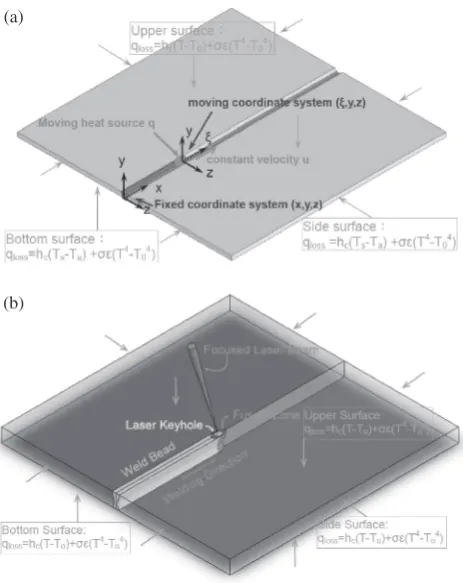
The analysis performed in this study considers the butt welding of two thin Alloy 690 plates of equal dimensions. During the welding process, the sheets are placed on a stationary work plane with the fixed coordinate system ðx;y;zÞshown in Fig. 1. The heat supplied to the weldment is provided by a GTAW (Fig. 1(a)) and a LBW (Fig. 1(b)). In each case, the moving heat source is modeled using the moving coordinate system ð;y;zÞand is assumed to have a Gaussian heat distribution. During the welding process, the heat source moves continuously in thex-direction of the work plane at a constant velocityu. Thus, the moving heat source q, the heat supplied to the weldment, can be modeled as qð;y;zÞ, in which ¼xþut. The corresponding heat transmission can be computed from eq. (2).

2.4 Initial and natural boundary conditions

The initial and natural boundary conditions imposed in the mathematical welding model comprise two parts. The following conditions apply:

2.4.1 Initial condition

Tðx;y;z;0Þ ¼T0ðx;y;zÞ; ð3Þ

(a)

(b)

2.4.2 Natural boundary condition

kn @T

@nþqþhcðTT0Þ þ"ðT 4_T4

0Þ ¼0; ð4Þ

where kn is thermal conductivity normal to the surface (W/m_C),h

c is the heat transfer coefficient for convection (W/m2_{C), T0 is the atmospheric temperature for the}

con-vention and/or radiation,is the Stefan-Boltzmann constant (W/m2_C4_{), and"is the radiation emissivity.}

2.5 Model of welding heat source

In modeling the GTAW, it is assumed that the electric arc forms a moving heat source with a double ellipsoid heat source within the weldment.7)_{In modeling the LBW welding} process, the laser beam forms a moving combined heat source (a double ellipsoid heat source plus a surface heat source9)_{) because of the effect of surface overlapping pulse} laser welding. The resulting heat distribution is described by the following function:

2.5.1 Gaussian surface heat flux distribution

qðx;z;tÞ ¼ 3Q c2exp

3½xþuðtÞ

c2

exp 3z

2

c2

; ð5Þ

whereQis the energy input rate (W) andcis the character-istic radius of the heat flux distribution (m).

2.5.2 Double ellipsoid heat source distribution

(1) Forward ellipsoid heat source distribution

qfðx;y;z;tÞ ¼

6pffiffiffi3ffQ abcpffiffiffie

3½xþuðxtÞ2_=a2

e3y2=b2e3z2=c2; ð6Þ

(2) Rear ellipsoid heat source distribution

qrðx;y;z;tÞ ¼

6pffiffiffi3frQ

abcpffiffiffie

3½xþuðxtÞx2_=a2

e3y2=b2e3z2=c2; ð7Þ

and

ffþfr¼2; ð8Þ

where Q= energy input rate (W), a, b and c are the characteristic radii of flux distribution (m), ff is the energy fraction of the forward part, and fr is the energy fraction of the rear part.

3. Experimental Procedure and Simulation

3.1 Welding experiments

The GTAW and LBW butt weldments were fabricated using Alloy 690 plates with a thickness of 3 mm, and the welding experiment follows the design reported by Lee and Wu.17)_{The chemical composition of the Alloy 690 plates is} summarized in Table 1. The as-received plates were ma-chined into specimens measuring 75150mm2 _(length width). The GTAW butt weld comprised two beveled Alloy 690 plates clamped in such a way as to form an 80_V-groove

with a 2.4 mm root opening gap and a 1 mm root face. The weldment was fabricated using a direct current straight polarity (DCSP) GTAW process and was accomplished using two welding passes. The welding process was performed using Alloy 52 filler metal wire with a core diameter of 2.4 mm. The composition of Alloy 52, as determined in accordance with the AWS A5.14 ERNiCr-7 specification, is

summarized in Table 2. The two welding passes were conducted using the process parameters shown in Table 3 with a pure argon (99.9%) shielding gas in both cases.

The LBW process was performed without filler metal, using a numerical control (NC) Rofin-Sinar CW025 Nd:YAG laser system with a maximum mean power of 2.5 kW. The weldments were fabricated with the laser system set in its pulse wave (PW) mode with a constant mean power of 1750 W, and a welding speed of 800 mm/min (see Table 3). The weldments were fabricated using pure nitrogen as both the face shielding gas (flow rate: 20 L/min) and the back shielding gas (flow rate: 10 L/min).

The temperature distributions within the GTAW and LBW weldments were measured continuously throughout the welding process using K-type thermocouples with a diameter of 0.127 mm (AWG No. 36). As shown in Figs. 2(a), 2(b) and 2(c), the thermocouples were attached to the lower surface of the weldments in order to avoid the effects of direct thermal radiation from the welding heat source and were arranged in such a way that the localized temperature gradients and thermal histories could be computed in various regions of interest within the weldment (e.g. the coarse grain zone, the weld decay zone, and the base metal). The thermocouple outputs were sampled every 100 ms and were saved to a PC for further processing.

3.2 Numerical simulation of GTAW and LBW welding processes

The temperature fields induced during the GTAW and LBW welding processes were simulated using ANSYS software based upon the time-step parameters given in Table 4 and the finite element models presented in Figs. 3(a) and 3(b). The two models were constructed using both eight-and twenty-nodal thermal conduction solid elements. In both cases, a fine mesh (3-D 20-node thermal element) was used in the regions of the weldment subject to a higher temperature gradient (i.e. close to the welding fusion line), while a coarse mesh (3-D eight node thermal element) was applied else-where. In practice, a finer mesh size is required to capture the temperature distribution induced by a smaller heat source.

Table 1 Chemical composition of Alloy 690 (mass%).

Ni Cr Fe Mn Ti C Si Cu P S Co

59.05 29.45 Bal. 0.29 0.28 0.019 0.33 0.02 0.01 0.001 0.014

Table 2 Chemical composition of Inconel Filler Metal 52 (I-52) (mass%).

Ni Cr Fe Mn Ti C Si Cu P S Al

60.39 28.91 8.89 0.25 0.51 0.03 0.16 0.01 0.003 0.001 0.64

Table 3 Welding parameters for GTAW and LBW weldments.

Voltage Current

Welding speed (mm/min)

GTAW (V) (A)

1st 15 90 84

2nd 15 90 108

LBW Waveform Average power (W) Welding speed (mm/min)

Thus, the GTAW weldment (with a relatively large spot size) was meshed using a grid comprising 56180 elements and 102669 nodes, while the LBW weldment (with a far smaller spot size) was meshed using a grid comprising 63225 elements and 115585 nodes. The function of Element Birth and Death was employed to simulate temperature field in filled metal GTA welding. In the simulations, the ambient temperature and initial workpiece temperature were both specified as 20C, and the heat convection coefficient between the weldment and the ambient environment was assumed to be 60 J_C/m2_{. Finally, the heat convection} coefficient between the weldment and the face shielding gas was specified as 120 J_C/m2_{. As discussed in Section 1, the} specific heat, thermal conductivity, and density of most engineering materials vary as a non-linear function of the temperature. Accordingly, in the present simulations, the thermal physical properties of the Alloy 690 plates and the I52 filler metal were specified in accordance with the profiles shown in Figs. 4(a) and 4(b), respectively, taken directly from the JMatPro database.

4. Results and Discussions

4.1 Cross-sectional morphology and sensitization region of the weldment

In accordance with the heat conduction formula given in

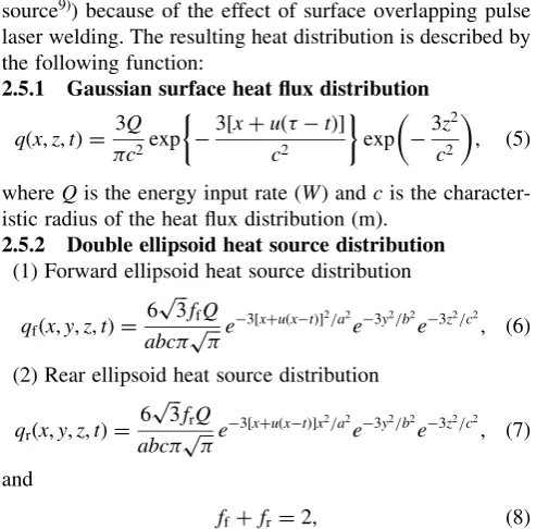
eq. (2), it can be seen that the temperature gradient within the weldment is determined by the thermal conductivity k, specific heatC, and density, which gained from Figs. 4(a) and 4(b). Figure 5(a) presents snapshots of the simulated temperature field within the 2nd pass GTAW weldment after the 680th s (left side), and shows the cross-sectional morphology of the corresponding experimental weld (right side). Note that in the simulation images, the red dotted line represents the temperature 1380_{C (i.e. the melting point of}

Alloy 69016)_{), and therefore the area above that (as indicated} by the above 1380_{C regions in Fig. 5(a)) corresponds to the}

fusion zone (FZ) of the 2nd pass weld. From inspection, the width of the weld root is found to be 5.6 mm. Figure 5(b) presents snapshots of the simulated temperature field within the LBW weldment after the 5.6th s (left side), and shows the cross-sectional morphology of the corresponding experimen-tal weld (right side), the weld root of which is approximately 1 mm. In other words, good agreement is observed between the two sets of results, and hence the validity of the numerical model in predicting the size of the weld cross-section is confirmed.

The color contours in the simulation images provide a convenient means of predicting the extent of the WDZ region within the weldment. For example, Fig. 6(a) presents the

(a)

(b)

(c)

Fig. 2 Schematic illustration showing temperature measurement positions (a) 1st pass of GTAW (b) 2nd pass of GTAW (c) LBW.

Table 4 Time-step data used in GTAW and LBW simulations.

Heat source travel speed (Experimental)

(mm/min)

Time-step (Simulation)

(mm)/(s)

Heat input (Experimental)

(J/mm)

Heat input (Simulation)

(J/mm)

GTAW 1st 84 (0.9)/(0.64) 964.3 540.43

2nd 108 (0.9)/(0.5) 750 396.05

LBW 800 (0.667)/(0.05) 131.25 98.1

(a)

(b)

transient temperature field of the 2nd pass of the GTA weldment, in which the green regions, corresponding to a temperature range of 6201020_{C, mark the extent of the}

WDZ region of the HAZ. In contrast, the three-dimensional SEM image18) _{presented in Fig. 6(b) shows that the WDZ} region of the weldment is susceptible to IGC. The WDZ region in the weldment has a width of around 4.4 mm (z¼4:08:4mm). Figure 6(c) shows the transient temper-ature field in LBW, which can be compared with the three-dimensional SEM image18) presented in Fig. 6(d). The green regions corresponding to a temperature range of

6201020C mark the extent of the WDZ region of the HAZ, and the WDZ region in the LBW weldment has a width of approximately 0.9 mm (z¼1:051:95mm). Figures 6(a) and 6(c) present the simulated transient temperature fields

within the GTAW and LBW weldments after the 680th and 5.6th s, respectively. It is clear that the LBW weldment has both a smaller HAZ and a narrower WDZ region.

4.2 Comparison of experiment and simulation

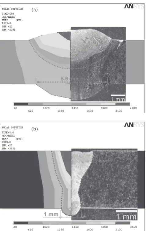
Figures 7(a) and 7(b) present the experimental and simu-lated thermal histories, respectively, for the three mainly measurement positions on the 1st and 2nd pass of the GTAW weldment. From the profiles corresponding to measurement positionsTG1andTG2in 7(a), located in the WDZ region of the weldment, it can be seen that the maximum experimental temperatures are 874.2 and 686.3_{C, while the corresponding}

simulation values are 889.7 and 680.15_{C. In the case of the}

experimental results forTG1andTG2in 7(a), the correspond-ing region of the weldment cools through the WDZ range in approximately 19.1 (i.e. (51.4–38.3)) and 12.1 (i.e. (48.8– 36.7)) s, and thus the cooling rates are found to be around 13.3 (i.e. (254.2/19.1)) and 5.5 (i.e. (66.3/12.1))C/s. In the case of the simulation results, the corresponding the cooling rates are 12.4 (i.e. (269.7/21.8)) and 4.6 (i.e. (60.15/ 13))C/s, and the time durations within the sensitization range are 21.8 (i.e. (135.4–113.6)) and 13 (i.e. (128.4– 115.4)) s. From the profiles corresponding to measurement

(a)

(b)

Fig. 4 Thermal properties of Alloy 690 base material and I52 filler metal:16)_{(a) Thermal properties of Alloy 690 (b) Thermal properties of} I52 filler metal.

(a)

(b)

positionsTG1,TG2andTG3in 7(b) located in the sensitization region of the weldment, we can see that the maximum experimental temperatures are 1024.3, 811.8 and 610.6_C,

while the corresponding simulation values are 1025.04, 745.2 and 620.6C. In the case of the experimental results forTG1 andTG2 in 7(a), the corresponding region of the weldment cools through the sensitization range in approximately 28.0 and 23.1 s, and thus the cooling rates are found to be around 14.3 and 8.3_{C/s. In the case of the simulation results, the} (a)

(b)

(c)

(d)

Fig. 6 Transient temperature field and three-dimensional SEM image of GTAW and LBW weldments: (a) Transient temperature field of the 2nd GTAW in simulation at 680th s (b) Three-dimensional SEM image of GTAW weldment18)_{(c) Transient temperature field of GTAW in} simu-lation at 5.6th s (d) Three-dimensional SEM image of LBW weldment.18)

(a)

(b)

(c)

corresponding cooling rates are 12.7 and 5.44_{C/s, and the}

time durations within the sensitization range are 31.5 and 23 s. In short, good agreement exists between the exper-imental and simulation results for both passes of the GTAW weldments. Although little differences do exist between the experimental cooling rates and the simulated cooling rates at temperature measurement positionsTG4,TG5andTG6, they do not require discussion because their positions are not in the WDZ zone.

Figure 7(c) presents the experimental and simulated thermal histories, respectively, for the four measurement positions on the LBW weldment. In Fig. 7(c), the peak experimental temperatures at measurement positions TL1 and TL2, both located within the sensitization region of the weldment, are found to be 1234.8_{C and 776.1C,}

respectively. Meanwhile, the corresponding regions at TL1 and TL2 of the weldment heat and cool through the sensitization range within 1.8 (i.e. (4.9–3.1)) s and 1.2 (i.e. (4.6–3.4)) s, respectively. Figure 7(c) shows that the peak simulated temperature values at measurement positionsTL1 andTL2are 1265 and 789.7C, respectively. The correspond-ing regions atTL1andTL2of the weldment cool through the sensitization range in approximately 1.6 (i.e. (12.1–10.5)) and 1.25 (i.e. (11.7–10.45)) s, respectively. From inspection, the simulation results for the peak temperature in the LBW weldment deviate from the experimental values by no more than 3%. Consequently, good agreement is observed between the experimental results and the simulation results for the temperature field at the measurement position.

Figure 8 presents the numerical and experimental results obtained for the peak temperature profiles within the GTAW and LBW weldments. The simulation results are computed using various values of the thermal physical property and are compared with the experimental measurements obtained at equivalent positions within the weldment. The welding speeds in the GTAW process (i.e. 84 mm/min in the first pass and 108 mm/min in the second pass, see Table 3) are significantly slower than that in the LBW process (i.e. 800 mm/min). Consequently, the GTAW weldment receives a greater heat input than the LBW weldment and cools more slowly, and the GTAW weldment has a smaller gradient than those of the LBW weldment. In addition, in Fig. 8, the curves labeled ‘‘k¼C’’ depict the simulation results obtained when computing the temperature field using constant values of the heat conduction coefficientk, specific heatC, and density derived at room temperature (20_{C). In other words, the three}

curves represent a linear rather than non-linear simulation result. It is observed that the two profiles for GTAW deviate to a greater or lesser extent from the experimental temper-ature fields. But for LBW, both approaches give roughly the same results, perhaps due to the much faster thermal cycle. The deviation of peak temperature in LBW is less than in GTAW because the welding speed of LBW is higher than GTAW. Thus, the importance of taking the temperature-dependent nature of the physical properties into account for a slower welding speed when simulating the welding process is confirmed.

Since, as shown in Fig. 8, the LBW weldment cools more rapidly than the GTAW weldment, it thus can be inferred that the LBW weldment has better IGC resistance than the

latter. Thus, the two figures confirm that the LBW process results in a lower total heat input to the weldment and a more rapid heating and cooling effect. As a result, the LBW weldment has both a narrower HAZ than the GTAW weldment and lower susceptibility to sensitization (i.e., better IGC resistance).

4.3 Calculation of time spent in sensitization region of weldments

As discussed in 4.1, Alloy 690 is particularly prone to sensitization at temperatures in the range6201020_{C. The}

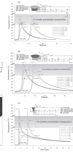
amount of carbide phase precipitated within the HAZ of the weldment, and thus the susceptibility of the weldment to IGC, depends on the time for which the weldment remains within this temperature range during the heating and cooling stages of the welding process. The improved corrosion resistance of the CGZ region is explained by its proximity to the FZ, where the local temperature exceeds 1020C during the welding process. As a consequence, the Cr-carbides microstructure dissolves within the matrix, rather than precipitating at the grain boundaries, thereby reducing the number of potential sites for IGC initiation.18)_{In general, we} can estimate durations of sensitization by experimental investigation, but it is not easy to estimate the locations of those critical points accurately of the WDZ such asTG1(see inset in Fig. 9(a)) and TLa (see inset in Fig. 9(b)). So, the simulation can help us to investigate the temperature profiles in the welding process. Fortunately for the GTAW weld, at positions TG1 and TG2, the length of time for which each measurement position remained within the sensitization range could be calculated directly. The durations for which the GTAW weldment is heating and cooling through the sensitization range are approximately 54.5(23+31.5) s atTG1 and 36(13+23) s atTG2, and thus the average cooling rates are found to be around 12.8 and 5C/s. Figure 9(b) presents the simulated thermal histories for LBW, at each of the considered measurement positions. The durations for which

the LBW weldment cools through the sensitization range are approximately 1.2 s atTL1, and those for heating and cooling through the sensitization range are 1.45 s atTLa and 1.2 s at TL2. Thus the average cooling rates are found to be around 333.3, 275.9, and 141.4_{C/s. Since the GTAW weldment}

spends relatively more time within the sensitization temper-ature range than LBW weldment, the average cooling rates of the HAZ in the GTAW weldment is lower than those of the LBW weldment. Consequently, the WDZ of the LBW weldment is significantly more resistant to IGC than the corresponding region of the GTAW weldment.

5. Conclusions

This study has performed a numerical investigation into the temperature fields induced within GTAW and LBW weldments in order to better understand their respective sensitization tendencies, utilizing a moving heat source model and the high-temperature physical property data derived using JMatPro software. The validity of the numer-ical model has been confirmed by comparing the simulation results with the corresponding experimental results. The major findings of this study can be summarized as follows:

(1) The calculated weld pool geometry, peak temperature and time duration within the sensitization range in different regions of the GTAW and LBW were in good

agreement with the corresponding experimental results for the welding of plates, indicating the validity of the modeling approach.

(2) When specifying the thermal physical property from the JMatPro database in the thermal welding model, the simulated temperature fields deviate less from the experimental temperature fields for GTAW. In LBW, however, due to the much faster thermal cycle, both approaches give roughly the same results.

(3) The simulated transient temperature fields provide a reliable and convenient means of estimating the range and size of the sensitization zone and the time duration of sensitization temperature in the GTAW and LBW weldments, especially in the case of the time duration or cooling rates in critical positions that are significantly susceptible to the effects of IGC.

Acknowledgments

The authors gratefully acknowledge the financial support of National Science Council, Taiwan (ROC), under Contract No. NSC 99-NU-E-006-001.

REFERENCES

1) P. M. Scott: An overview of materials degradation by stress corrosion in PWRs, Ed. by D. Fe´ron, CEA-Saclay and J-M Olive Corrosion Issues in Light Water Reactors: Stress Corrosion Cracking, (Woodhead England, 2007) pp. 3–24.

2) D. L. Harrod, R. E. Gold and R. J. Jacko: JOM53(2001) 14–17. 3) J. D. Kim and J. H. Moon: Corros. Sci.46(2004) 807–818. 4) H. T. Lee and J. L. Wu: Corros. Sci.51(2009) 733–743.

5) J. D. Kim, C. J. Kim and C. M. Chung: J. Mater. Process. Technol.114

(2001) 51–56.

6) D. Rosenthal: Trans ASME68(1946) 849–866.

7) V. Pavelic, R. Tanbakuchi, O. A. Uyehara and P. S. Myers: WJ Supplements48(1969) 295s–305s.

8) E. Friedman: J. Pressure Vessel Technol. Trans. ASME97(1975) 206– 213.

9) G. W. Krutz and L. J. Segerlind: WJ. Supplements57(1978) 211s– 216s.

10) J. Goldar, A. Chakravarti and M. Bibby: Metall. Trans. B15(1984) June 299–305.

11) A. P. Mackwood and R. C. Crafer: Opt. Laser Technol. 37(2005) 99–115.

12) F. Lu, S. Yao, S. Lou and Y. Li: Comput. Mater. Sci.29(2004) 371– 378.

13) X. Y. Shan, M. J. Tan and N. P. O’Dowd: J. Mater. Process. Technol.

192(2007) 497–503.

14) H. C. Kuo and L. J. Wu: J. Mater. Process. Technol.120(2002) 151– 168.

15) G. H. Little and A. G. Kamtekar: Comput. Struct.68(1998) 157–165. 16) JMatPro 4.1, Thermotech Sente Software 2007. Available from:http://

www.Thermo-tech.co.uk/.

17) H. T. Lee and J. L. Wu: Corros. Sci.51(2009) 439–445. 18) H. T. Lee and J. L. Wu: Corros. Sci.52(2010) 1545–1550. 19) T. Y. Kuo and H. T. Lee: Mater. Sci. Eng. A338(2002) 202–212. 20) H. T. Lee, Y. D. Lin, T. Y. Kuo and S. L. Jeng: Mater. Trans.48(2007)

1538–1547.

21) H. T. Lee, C. T. Chen and J. L. Wu: J. Mater. Process. Technol.210

(2010) 1636–1645.

22) H. T. Lee, C. T. Chen and J. L. Wu: Sci. Technol. Weld. Join.15(2010) 605–612.

23) ANSYS, Inc, Southpointe 275 Technology Drive Canonsburg, PA 15317.

(a)

(b)